Named by Pierre–Gilles de Gennes in his Nobel Prize lecture,^[1,2] “soft matter” vaguely refers to a wide spectrum of condensed materials, ranging from polymers, complex liquids, liquid crystals to foams, colloids, gels, granular materials, and biological materials. Various soft materials share some common features, such as significant entropic effect, large fluctuations, sensitivity to thermodynamic conditions (particularly a weak force can induce a large transformation), mesoscopic characteristic spatial and temporal scales, and the ability of self-assembly.^[3] Despite successes in some individual fields, such as polymers^[4] and liquid crystals,^[5] no general quantitative definitions have yet been provided for soft matter, and the intrinsic mechanisms leading to their common features are unclear.

Regarding the subtle balance between entropy and enthalpy contributions in soft matter, the term “entropy–enthalpy compensation” has been frequently carried out since 1950s, aiming to quantitatively describe the unique characteristics of soft matter (see, e.g., Refs. ^[6–14]). Initially, entropy–enthalpy compensation was referred to the phenomenon that a change in thermodynamic condition leads to almost identical changes in entropy and enthalpy, for the Helmholtz free energy or for the Gibbs free energy , where T is the system temperature, U is the system total energy, H is the system enthalpy, and S is the system entropy. In the term “entropy–enthalpy compensation”, “entropy” refers to , the entropic effect caused by a finite temperature and/or finite spatial degrees of freedom, and “enthalpy” refers (not rigorously) to interactions among particles, either U or H, for the sake of simplicity. However, this interpretation was doubted very likely an artifact caused by inappropriate data analysis methods.^[15,16] Recently, entropy–enthalpy compensation has taken another form of

(1)

(2)

The physical interpretation of this form is that the free energy cost or for a certain statistical process remains roughly unchanged when the thermodynamic condition changes, attributed to the compensated entropy change with respect to the enthalpy change. Another term “entropy–enthalpy balance” vaguely refers to the phenomenon that entropy and enthalpy have comparable contributions under a certain thermodynamic condition (see, e.g., Refs. ^[17–22]), yet frequently it takes the same expression as Eq. (1) or (2).

The current forms of the above two terms, however, neither reveal the statistical physics essence of soft matter nor provide a systematic explanation of the common features soft materials exhibit. The problem may reside in the fact that different thermodynamic states are compared to looking for the balance or compensation between thermodynamic entropy and enthalpy. Instead, in this paper, we will show that the balanced condition is satisfied in a single thermodynamic state, whose substates along an order parameter (or more general a reaction coordinate) have various ratios of entropy and enthalpy contributions rather than thermodynamic variables of entropy or enthalpy. By looking into the substates of the free energy landscape along a predefined order parameter, we will define soft matter as the materials working in the vicinity of a moderate point, at which entropy and enthalpy contributions among substates are well balanced (or have a minimal difference when the exact balanced condition cannot be satisfied). This (quasi-)balanced condition leads to the maximization of the order parameter fluctuation around the moderate point, which explains the intrinsic large fluctuation of soft matter. The associated response function also maximizes around the moderate point, which explains the sensitivity of soft materials to thermodynamic conditions. Their mesoscopic temporal and spatial scales may be explained by the maximization of the finite spatial correlation length around the moderate point. For convenience, we will call our theory the moderation theory.

From now on, we assume that by default the system is in the canonical ensemble, and “enthalpy” actually refers to the system total energy. The essential idea of the moderation theory is that the subtle balance between the entropy and enthalpy contributions of soft matter should be reflected by the probability distribution (or equivalently the free energy landscape) of all substates of a thermodynamic state (a state point in the phase space). With an appropriately defined order parameter, a thermodynamic system with very high dimensions (e.g., a system with N particles in the 3-D space has 6N degrees of freedom) is projected into a reduced phase space spanned by the order parameter. Note that here “substates” are microstates in the reduced phase space, not in the original full-dimensional space. For simplicity, in this paper, only the case with one order parameter h is considered, along with a generalized field B conjugated with h. Nevertheless, it should be straightforward to generalize the theory to the cases with multiple order parameters.

2.1. Free energy landscape

The Helmholtz free energy of a thermodynamic state point is

(3)

where with being the Boltzmann constant, and Z is the total partition function. In the reduced phase space spanned by an order parameter h, a substate has the probability density of

(4)

where is the partial partition function with the density of states and the energy. The free energy of a substate can be defined as

(5)

Note that and but . The free energy landscape of a state point along this order parameter is a collection of the free energies of all its substates. Note that B is conjugate to the order parameter h, and does not necessarily have to be a real external field.

2.2. Two-substate model

Without considering the generalized field B, for the simplest case of a classical statistical system with only two substates: entropy-dominated state 1 and enthalpy-dominated state 2 after projecting into the phase space spanned by an order parameter h, if the system energies of the two substates are U₁ and U₂ with , the densities of states are g₁ and g₂ with , and the associated order parameters are h₁ and h₂, then the system partition function is given by , where , i= 1 or 2, and the appearance probability . The free energies associated with the two substates are , or 2. At low temperatures, , the system is enthalpy-dominated; at high temperatures, , the system is entropy-dominated. Therefore, it is natural to require

(6)

at the moderate point when the system has the entropy and enthalpy contributions well balanced, which determines the temperature at the moderate point

(7)

If the generalized field B is considered with and , in some cases the two substates cannot have exactly balanced entropy and enthalpy contributions when varying B at a fixed temperature. Therefore, instead of requiring , we now define the moderate point as the one satisfying a looser condition,

(8)

where is the smallest free-energy difference taken at the moderate point , which is determined by the mathematical feature of and . To differentiate, the point satisfying (i.e., will be called the exact moderate point, otherwise it will be called the general moderate point, and the corresponding conditions are the exact moderate condition and the general moderate condition, respectively.

In Appendix A, we prove that the order parameter fluctuation maximizes at either the exact moderate point or the general moderate point for the two-substate model, where and .

2.3. Continuous case

When the substates are continuous, it is unobvious what kind of probability distributions have balanced entropy and enthalpy contributions. Our strategy is dividing the whole probability distribution into two parts by the ensemble average (expected value) of the order parameter : one side is entropy-dominated and the other side is enthalpy-dominated. As derived in Appendix B, based on the exact moderate condition for the two-substate model given by Eq. (6), we obtain the exact moderate condition for the continuous case

(9)

where and is the median satisfying . The general moderate condition is

(10)

where is the smallest possible deviation of the integral from 0 determined by the mathematical feature of . Note that when the difference between the entropy and enthalpy contributions is too large, it is unreasonable to still treat the system as a soft material. Nevertheless, usually the difference varies continuously with thermodynamic variables (e.g., temperature), and there are no natural boundaries distinguishing the “soft” region from other cases, a problem similar to the definition of the exact glass transition point.

As shown in Appendix C, the maximization of the order parameter fluctuation D_h with respect to the generalized field B has to satisfy

(11)

Under the assumption that the system energy U linearly depends on h, the condition for the maximization of D_h with respect to the temperature T (or equivalently is also Eq. (11). In Appendix D, we prove that the moderate condition given by Eq. (10) naturally leads to Eq. (11). That is, the order parameter fluctuation D_h maximizes at either the exact moderate point or the general moderate point for the continuous case.

2.4. Response function and spatial correlation length

In the linear response regime, the system Hamiltonian under a generalized field B can be written as

(12)

where U₀ is independent of B, and the probability density function should have the form

(13)

Since the total free energy is , the ensemble average of the order parameter

(14)

The response function corresponding to B is

(15)

where the order parameter fluctuation usually depends on both β and B.

According to Eq. (15), when varying the generalized field B at a fixed β, the response function maximizes exactly at the point D_h maximizes. When varying the temperature T (equivalently , this relation does not hold, but numerically the maximization of the response function appears at a point very close to the maximization of D_h if D_h varies slowly around its maximal point, as demonstrated in Appendix E.

The characteristic spatial scale can be quantified by the spatial correlation length. In the linear response regime, the spatial correlation length can be related to the response function as

(16)

where r is the spatial interval, , and the partial order parameter satisfies

(17)

In Appendix F, we show that the spatial correlation length maximizes when D_h maximizes. On the other hand, no quantitative connections can be established between D_h and the time correlation length, but as a rule of thumb, in view of the vast scale, for material systems, a larger spatial scale roughly corresponds to a longer temporal scale. This might explain why soft materials generally have mesoscopic characteristic spatial and temporal scales, since microscopic scales correspond to short correlation lengths and macroscopic scales correspond to divergent correlation lengths, while soft materials work under a thermodynamic condition in between.

The validity of the moderation theory was examined with a simplified polypeptide aggregation model. Previously, we simulated by coarse-grained molecular dynamics the aggregation behaviour of polyglutamine molecules in aqueous solution.^[23,24] We found that, in equilibrium, the instantaneous configurations of polyglutamine molecules fluctuate from distributing almost uniformly to aggregating very tightly, and the degree of aggregation decreases monotonically with temperature but first increases and then decreases with concentration. Based on the simulation data, we then projected this high-dimensional system into a one-dimensional phase space spanned by the so-called heterogeneity order parameter (HOP).^[25] characterizing the degree of aggregation, defined as

(18)

(19)

Since the momentum space is independent of the configurational space, is always cancelled out and only should be considered during normalization.

For the system with 27 32-residue polyglutamines, by fitting the simulation data, we determine the density of states

(20)

(21)

(22)

The generalized field associated with h is

(23)

(24)

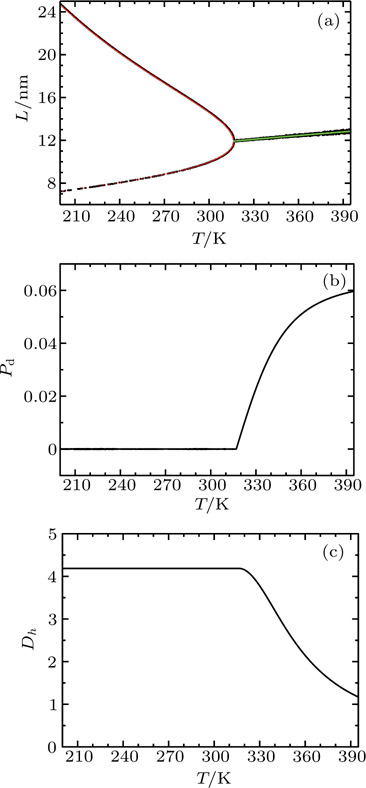
In this model, the fluctuation of the order parameter is a function of both temperature and concentration . In Fig. 1(a), the red line depicts the thermodynamic states at which takes the largest possible value of 4.1869. It is interesting to see that, below the critical temperature K, each has two corresponding L values, resembling the liquid-vapour phase transition of a finite-size system. For temperatures above , D_h cannot be as large as 4.1869, and the thermodynamic states with the largest D_h are drawn with a green line. In the same plot, the thermodynamic states determined by Eq. (10) are drawn with black lines, which almost perfectly overlap with the red and green lines, indicating that the order parameter fluctuations maximize at the moderate points. As shown in figs. 1(b) and 1(c), below , the entropy and enthalpy contributions are perfectly balanced at the exact moderate point and the maximal D_h always takes the largest possible value of 4.1869; above , with increasing temperature, the entropy contribution becomes larger and larger than the enthalpy contribution, and the maximal D_h at the general moderate point becomes smaller and smaller.

Fig. 1.

	Figure Option ViewDownloadNew Window
	Fig. 1. (a) Thermodynamic states with the largest fluctuation of the order parameter (red and green lines) and the moderate points determined by Eq. (10) (black lines). (b) Smallest probability difference defined in Eq. (10) as a function of temperature. (c) The largest order parameter fluctuation as a function of temperature.

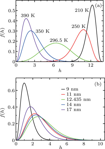
The probability density distributions at an arbitrarily chosen concentration nm and various temperatures are plotted in Fig. 2(a). According to Fig. 1, the moderate-point temperature at this concentration is K. At the low temperatures of 210 K and 250 K, due to the dominated enthalpy contribution, polyglutamine molecules aggregate tightly, leading to larger probabilities for larger h values. In contrast, smaller h values have larger probabilities at the high temperatures of 350 K and 390 K when the entropy effect dominates. In between, at the moderate point K, the distribution of is almost symmetric, resulting in the largest HOP fluctuation near this point.

Fig. 2.

	Figure Option ViewDownloadNew Window
	Fig. 2. Probability density distributions at (a) nm and various temperatures, and (b) K and various concentrations.

For a fixed temperature, varying L can also change the balance between entropy and enthalpy. The distributions at an arbitrarily selected K and various concentrations are plotted in Fig. 2(b). According to Fig. 1, the corresponding moderate-point box size nm, at which is broader than the distributions at any other concentrations by satisfying Eq. (10), although it is still asymmetric.

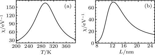
The response function χ corresponding to h has been calculated according to Eq. (15) and are shown in Fig. 3. As shown in Fig. 3(a), at nm also exhibits a peak, but the corresponding temperature is 292.7 K, slightly different from K due to the prefactor β. On the other hand, it is not surprising that at K, χ reaches its maximum at the moderate point nm (Fig. 3(b)), since the prefactor β is now a fixed value. Maximization of the response function around the moderate point manifests that, in the vicinity of the moderate point, a small change in the generalized field conjugate to the order parameter results in a large change of the order parameter. In other words, the system is very sensitive to the change of thermodynamic conditions. Two examples are the sensitivity of peptide self-assembly to temperature change.^[26,27] and the sensitivity of ionic liquid properties to molecular structure.^[28,29]

Fig. 3.

	Figure Option ViewDownloadNew Window
	Fig. 3. Response functions at (a) nm as a function of temperature and (b) K as a function of concentration.

The moderation theory should be quite general and should be able to be applied to most (if not all) soft materials. A possible application of the two-substate model moderation theory could be the case of chemical bond breaking and reformation. If all microsates of a chemical bond can be grouped into only two substates independent of temperature: the enthalpy-dominated connected state and the entropy-dominated broken state, then at the moderate temperature given by Eq. (7), the chemical bond has equal probabilities of being connected or broken. Well above the moderate temperature, the bond is broken most of the time due to thermal fluctuation, and is connected most of the time well below the moderate temperature. This simplified picture might be helpful for understanding the functions of hydrogen bonds in biological systems.

Another possible application is the determination of the best working temperature of biochannels. A biochannel works the best when the difference between the open state and the close state, modulated by a binary variable (e.g., binding and unbinding of an ion on a specific binding site) or B₁, is the largest. If we choose the width of the channel to be the order parameter h, the difference is

(25)

If the system energy U linearly depends on h, the maximization requirement leads to the condition at the moderate point

(26)

Alternatively, integrating the first part of Eq. (15) leads to

(27)

Along with the second part of Eq. (15), we obtain

(28)

Either Eq. (26) or Eq. (28) can be used to determine the best working temperature of a biochannel.

In summary, we developed the moderation theory for soft matter by defining the moderate point of a statistical system at which the entropy and enthalpy contributions among substates along an order parameter perfectly balance each other or have a minimal possible difference. The order parameter fluctuation maximizes around the moderate point. Soft materials work in the vicinity of the moderate point, which explains their sensitivity to thermodynamic condition changes via the relation between the order parameter fluctuation and the associated response function. The mesoscopic characteristic spatial and temporal scales of soft matter are also explained by the maximization of the finite spatial correlation length at the moderate point. The moderation theory was validated by the simplified statistical model for polyglutamine aggregation, and its possible applications to switching chemical bonds and biochannels were also briefly discussed. The moderation theory is anticipated to form the basis of the theoretical framework providing a quantitative definition for soft matter.

An important feature of the moderation theory is that the moderate point heavily depends on the order parameter because a specific choice of an order parameter reflects the perspective of the study for a given soft material. In addition, it is worth emphasizing that, the maximization of the response function is not always exactly at the moderate point, and there are no distinct boundaries for the entropy and enthalpy difference dividing the “soft” and “non-soft” regions of the system, reflecting the “softness” feature of soft matter.

More questions related to the moderation theory for soft matter are open for investigation. Figure 1 demonstrates that the polyglutamine aggregation model resembles a liquid–gas phase transition of a finite-size system, and the line above the critical temperature is very likely the so-called Widom line.^[30–32] Therefore, the relations between the moderation theory and the phase transition of a finite-size system as well as the Widom line are worth investigating. In addition, it is interesting to see how the current terminologies of entropy–enthalpy compensation and entropy–enthalpy balance fit in the moderation theory. Finally, the moderation theory might help to explain why soft matter can self-assemble into ordered structures, a unique feature of soft matter very important in various scientific areas including physics, chemistry, biology, and materials science.