In comparison with x-ray absorption imaging, x-ray phase contrast imaging (XPCI) — a technique that utilizes x-ray phase shift for the detection of weakly absorbing materials — can provide much better contrast-enhanced images.^[1–4] Since Pfeiffer first proposed XPCI based on the Talbot–Lau interferometer with low-brilliance x-ray sources,^[5–10] it has developed rapidly, and attracted much attention over the past decade. In the detector plane of Talbot–Lau interferometer, however, the self-images period of the phase grating is much smaller than the detector pixel size, which results in difficulty in detecting. This is resolved by introducing an analyzer grating, which forms the Moiré fringes with the self-image of the phase grating. These Moiré fringes can magnify the x-ray deviations, typically of the order of a few micrometers. A high aspect-ratio absorption grating is necessary to increase the visibility of the Moiré fringes, but is difficult to achieve in practice, especially for the analyzer gratings. In 2011, Momose et al. implemented the XPCI based on the inverse geometry of Talbot–Lau interferometer without an analyzer grating.^[11] However, the system length (7 m) makes the practical applications impossible. Morimoto et al. used the multiline copper targets embedded in a diamond substrate to implement XPCI within 1 m source-detector distance in 2014.^[12] Note that this system would have a longer system length if used with higher energy x-rays, which would lead to difficulty in being used practically. In 2009, Huang proposed XCPI based on geometrical optics. It broke through the coherence length limitation. But to some extent, it lacked flexibility.^[13] X-ray phase contrast imaging seems to run into the bottleneck on its advanced ways to practical applications and we have found solutions for some constraints.

In the Talbot–Lau interferometer, Moiré fringes are formed by the self-images of the phase grating and the analyzer grating. When the x-rays pass through an object, the detector can determine the tiny deviated angles magnified by the Moiré fringes. However, when we retrieve signals by phase-step methods, we do not see any magnification factors related to Moiré fringes. Therefore, we have enough reason to doubt the actual function of the analyzer grating. We will find the answer through the forming process of the shifting curves in the Talbot–Lau interferometer.

Figure 1(a) shows the Talbot–Lau interferometer setup. The setup consists of an x-ray tube source, a source grating G ₀, a phase grating G ₁, and an analyzer grating G ₂. The G ₀–G ₁ distance, z ₁, is larger than G ₁–G ₂ distance, z ₂. As shown in Fig. 1(b), self-images of G ₁ and analyzer grating G ₂ have the same period. In a pixel, the signals — the integrated intensity transmitted through the analyzer grating — contributed by different fringes are the same. Therefore, we need only consider the integration of a single fringe period, which is shown in Fig. 2.

Fig. 1.

	Figure Option ViewDownloadNew Window
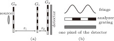	Fig. 1. Schematic diagrams for a Talbot–Lau interferometer. (a) The experimental setup. (b) The intensity detection principle.

Fig. 2.

	Figure Option ViewDownloadNew Window
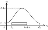
	Fig. 2. The schematic diagram of the integration effect in the one fringe period.

In Fig. 2, A, d ₂, and c represent the amplitude, period, and average intensity of the fringe, respectively. The transmitted area length in one period of G ₂ is b, and b ₀ represents the relative position between G ₂ and the fringe. The light-proof area of G ₂ is not shown in Fig. 2.

The signal that one pixel acquires can be quantified by

(1)

The setup in Fig. 3(a) consists of a micro-focus source 5 μm in diameter, an absorption grating with a 42-μm period and a detector with a 74.8-μm pixel size. In Fig. 3(b), one fringe period corresponds to three pixels in the detector plane, and the 224.4-μm fringe period can be deduced. Figure 3(c) displays an experimental shifting curve with a 13.6% visibility and figure 3(d) shows the experimental intensity fringes with poor definition. In this experiment, Moiré fringes are nonexistent due to no analyzer grating. In other words, the shifting curves are unrelated to the Moiré fringes but directly originate from the detector integration effect. By utilizing the detector integration effect, it is not necessary to magnify the grating self-image to a level that is large enough to be resolved directly by the detector in inverse geometry of Talbot–Lau interferometer. Therefore, both the system length and the exposure time can be reduced. For example, the system length can be scaled down to 2.1 m in the system designed by Momose et al.,^[11] and the intensity can be increased by 10 times by utilizing the schematic diagram shown in Fig. 3(b). In the above setup, we can also employ a detector with large pixels and large field of view. It will greatly reduce noise, which is related to mechanical vibration.

Fig. 3.

	Figure Option ViewDownloadNew Window
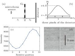	Fig. 3. (color online) (a) Experimental setup based on the geometrical optics that does not have an analyzer grating. (b) The principle of the detector integration effect. (c) An experimental shifting curve. (d) The experimental intensity fringes.

Using the setup described above, we reconstruct the absorption and differential phase images of PE through the detector integration effect. The experiment is carried out at 40 kV/80 μA with a 1-m system length. The PE diameter is 15 mm, and the distance from the object to the detector is 41.5 cm. Ten raw images, each with a 20-s exposure time, taken at different positions from the absorption grating, are used to obtain the absorption and differential phase images. In order to reduce the exposure time and noise, an x-ray tube source and a source grating can be used in combination with increased current intensity instead of a micro-focus source. By comparison with Fig. 4(a), the image in Fig. 4(b) still maintains the edge-enhanced characteristic. Two strong signal peaks are clearly visible in Fig. 4(d) while no signal peaks at the edge of PE are visible in Fig. 4(c). Note that the noise in Fig. 4, can be further reduced through the use of better quality gratings. In conclusion, figure 4 confirms that the x-ray phase contrast imaging based on geometrical optics with large period absorption gratings, which will improve the system mechanical stability, is feasible, and the setup is simple due to the lack of an analyzer grating.

Fig. 4.

	Figure Option ViewDownloadNew Window
	Fig. 4. (color online) (a) A reconstructed absorption image of PE. (b) A reconstructed differential phase image of PE. (c) The cross-section of the black rectangle in panel (a). (d) The cross-section of the black rectangle in panel (b).

There is a surprising detail we should mention, i.e., all the experiments above are confirmative experiments, and are done with a 25% duty cycle source grating. This means that the source grating light-proof area is three times larger than the source grating transmission area in one period. Conventional absorption grating used as a projective grating has a 50% duty cycle. If we use an absorption grating with a 25% duty cycle as a projective grating, its height can be improved by 50% under the condition of the same aspect ratio. This indicates that such an absorption grating can absorb much higher energy x-rays and much higher x-ray energy is available for imaging.

The main disadvantage of the method proposed here is the relatively poor shifting curve visibility. An alternative solution has been found through the following experiment. The visibility given by formula (1) is

(2)

Fig. 5.

	Figure Option ViewDownloadNew Window
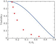	Fig. 5. (color online) Shifting curve visibilities as a function of b/d 2. The blue curve represents the theoretical results and the star marks represent the experimental results. A/c is fixed at 0.5.

Although experimental values fit the theoretical values poorly, the visibility change trend along with a decrease in b/d ₂ inspires us to increase the shifting curve visibility by reducing the effective illumination area of the detector pixels,^[14] which is equivalent to reducing b. This phenomenon is well-understood. When the effective illumination area of the pixels is reduced, the average shifting curve intensity is reduced and the visibility is increased. Another way to increase the visibility is to reduce the average intensity of the grating self-image. This indicates that c, in formula (2), should be reduced as much as possible.

When a detector with an appropriate resolution and field of view is chosen, an analyzer grating with the same detector period will reduce the effective pixel illumination area. For example, we can use an analyzer grating with a 74.8-μm period, and a 50% or other duty cycle, in the above experiments. It is obvious that the fabrications of such large period gratings are easier than those of conventional analyzer gratings with a few micrometers periods.^[15–17]

If an analyzer grating is used, we suggest that the optimal fringe period is equal to the detector period. When the fringe period is less than the detector period, each fringe period corresponds to a deviated angle of the x-rays. The deviated angle that one pixel can detect is the average of all deviated angles from different fringes in one pixel. However, the small fringe period will increase the system instability. On the contrary, when the fringe period is larger than the detector period, the minimum detectable deviated angle will rapidly increase. Therefore, when the fringe period is equal to the detector period, the influence of mechanical vibration will be reduced and detector resolution can be fully utilized in the meantime.

In this work, through the investigation of the shifting curve formation process, we proposed an alternative method to acquire shifting curves by using the detector integration effect. The principle of shifting curves based on the detector integration effect originates from the method that acquires shifting curves in the Talbot–Lau interferometer. In practical applications, we not only take advantage of inverse geometry of Talbot–Lau interferometer but also avoid overlong system length in the meantime. This method can shorten the system length, is applicable to large period gratings, and can use the detectors with large pixels and large field of view. We also find that absorption gratings with a duty cycle less than 50% can be utilized effectively, which will result in higher x-ray energy available. Finally, through the use of a large period analyzer grating matched detector pixel size, we can effectively improve the shifting curve visibility. The optimal fringe period is also given.