Optimizing calculation of phase screen distribution with minimum condition along an inhomogeneous turbulent path
Shao Wen-Yi1, 2, 3, Xian Hao1, 3, †,
Key Laboratory on Adaptive Optics, Chinese Academy of Sciences, Chengdu 610209, China
Institute of Optics and Electronic, Chinese Academy of Sciences, Chengdu 610209, China
University of Chinese Academy of Sciences, Beijing 100049, China


† Corresponding author. E-mail: xianhao@ioe.ac.cn

Project supported by the National Natural Science Foundation of China (Grant No. 61308082).

Abstract
Abstract

When building an experimental platform for light propagation along an inhomogeneous turbulent path, it is very essential to set up the reasonable distribution of phase screen. Based on multi-layered model of phase screen, an iterative optimization algorithm of phase screen position is given in this paper. Thereafter, the optimal position of phase screens is calculated under the Hufnagel–Valley5/7 and Hefei-day turbulence profile. The results show that the positions of phase screen calculated by the iterative algorithm can fit well with the turbulence profile rather than mechanically placed phase screens at equal distance. Compared with the uniform distribution of phase screens position, the residual phase error of the iterative algorithm decreases very significantly. The similarity degree between them is minimal when number of layers is equal to two.

1. Introduction

Atmospheric optical communication has been receiving considerable attention recently for providing secure, low-cost, rapidly deployable, dynamic data transmission at very high rates.[1] However, owing to inhomogeneity in the temperature and pressure of the atmosphere, the refractive index varies along the optical path, which in turn leads to angle-of-arrival fluctuations, intensity fluctuations, and beam broadening.[2,3] Thus, these deleterious effects of turbulence severely limit the performance of the laser communication system.

At present, a method for modeling laser beam propagation in a turbulent atmosphere by using thin phase screens along the propagation path has been studied extensively.[46] In the laboratory, this method can be served as a guidance for building an experimental platform for light propagation along an inhomogeneous turbulent path. The most commonly used equipment of simulating atmospheric turbulence is based on liquid-crystal spatial light modulators (SLM) and rotating glass plate, which act as the phase screen. Considering the high expenses of these experimental device, it would not be possible to set up too many phase screens in the experiment. Meanwhile, when laser beam propagation along the nearly horizontal path where the atmospheric structure constant of the refractive index is approximately equal to be constant, discrete phase screens are always distributed uniformly. But with the consideration of the vertical and sloping paths through a turbulent atmosphere, the strength of turbulence is a function of height, wind speed and meteorological parameters. If the uniform distribution of phase screens is still used in this case, the effects of atmospheric turbulence could not be simulated accurately. So a reasonable distribution of phase screens becomes very necessary. Schmidt et al. explored the effective position distribution of phase screens to avoid unnecessary complexity in the laboratory setup.[7] His method is based on the situation that one phase screen is located in the transmitter plane and the other half way to the receiver. Phillips et al. introduced different schemes of phase screen distribution in order to achieve certain values of the Rytov variance.[8] Qian et al. outlined three different methods: uniformly distributed phase screen, equivalent Rytov index-interval phase screen and equivalent Fried parameter-interval phase screen.[9] In addition, Fusco et al. presented that small number of equivalent layers (2 or 3) is required to obtain an accurate restitution of the phase in a large field of view.[10] But both efforts do not solve the problem of the position distribution of phase screens along an inhomogeneous turbulent path systematically, which means that a suitable mathematical physical model has not been put forward to solve it. Moreover, personal subjectivity in choosing the position and number of phase screens may increase uncertainty of experimental results. In our case, a number of phase screens are placed along 11 meters of light propagation path in the experimental platform to simulate the effect of atmospheric turbulence within 10 km. Although a large number of phase screens are applied in the numerical simulation, it cannot be achieved in the laboratory limited by experimental funds. So it is very necessary to explore the phase screen distribution with minimum condition along an inhomogeneous turbulent path.

In this paper, based on the multilayer model of atmospheric turbulence, an iterative optimization algorithm of phase screen position is investigated. Meanwhile, under condition of the Hufnagel–Valley5/7 and Hefei-day atmospheric turbulence profile model, the optimal distribution of phase screens and the boundary of atmospheric discrete layers are calculated respectively. The minimum condition of phase screen distribution are also introduced by the analysis of similarity degree.

2. Principles and methods
2.1. Position distribution model of multiple phase screens

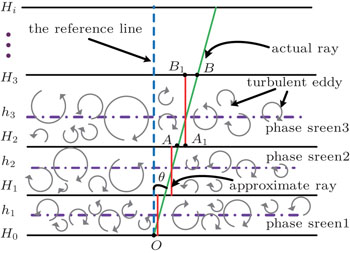
The atmospheric turbulence is modeled as a series of thin phase screens, as shown in Fig. 1. In the model, the volume turbulence is divided into N sections, each of which has the upper and lower bounds. Hi−1 and Hi are the lower and upper bounds of i-th section, respectively. hi is the position of phase screens. The actual laser beam propagates from point B to point O (green line).

Fig. 1. Schematic diagram of the multilayer model of atmospheric turbulence.

The angle θ between the actual laser beam (green line) and the approximate one (red line) is very small. Thus we assume that the strength of the turbulence varies little along the horizontal direction. The optical path difference (OPD) between them is given by[11]

where n(r,h) is the index of refraction at position r and altitude h, (r,h) is the approximate value to the index of refraction at position r and altitude h. Because the perturbations to the refractive index of each section is concentrated in the single phase screen, (r+θh,h) can be expressed as

where δ(h) represents the Dirac delta function. It has the fundamental property that

By integrating both sides of Eq. (2) with respect to h, then

By substituting Eq. (4) into Eq. (1), it gives

The relationship between phase difference Δϕ and optical path difference ΔLOPD can be described as

where k = 2π/λ is the wave number. Consequently, Δϕ can be written as

where ϕ̃ and ϕ represents the wavefront phase of approximate laser beam and actual one, respectively.

From Eq. (7), we can obtain the variance of Δϕ such that

Under the Kolmogorov model, the most commonly used length scale is the Fried parameter r0. The 2D phase structure function in this case is

where Δr = rr′ is the distance between the two points. For a plane wave, the atmospheric coherence diameter

The phase structure function can be expressed as

where laser beam propagates from point B to point O, and L is the propagation distance. is known as the atmospheric refractive index structure parameter. Substituting Eq. (10) into Eq. (11), one can obtain

Consolidating Eqs. (9) and (12) into Eq. (8) enables us to compactly express the variance of Δϕ (residual phase error) as

2.2. Iterative optimization algorithm

In order to assure that the effects of discrete phase screens match those of the atmospheric turbulence in reality best, the variance of residual phase error needs to be minimized. Using Eq. (13), we can get the derivation of Hi and hi respectively[11]

where

Setting Eqs. (14) and (15) to zero can give us the optimization conditions for a minimum of

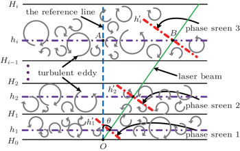
When the angle between the actual laser beam and the hypothetical one becomes very large, the optimal positions of discrete phase screens (hi) are required to be revised. In Fig. 2, ΔOAB is a right-angled triangle, is the revised positions of discrete phase screens. The relationship between hi and can be written as

In order to better illustrate the principles of the iterative algorithm, we describe the basic steps as follows:

Step 1 set initial value of H0, h1, and N. In our case, H0 = 0, h1 = 100 m, and i = 1,2,3,…,N.

Step 2 calculate the value of . Owing to the volume turbulence is divided into N sections, we need to obtain the value of R1 firstly when i = 1.

Step 3 estimate the value of H1 and evaluate the value of . If |RiTi| < p (p is the error limit), the value of H1 satisfies Eq. (18). Otherwise, H1 = H1 +1. This process repeats until Eq. (18) is satisfied. Considering the speed of numerical calculation, we choose that H1 = 1000 m and p = 0.05 ∼ 0.09 in our case.

Step 4 calculate the value of h2 using Eq. (17). Thereafter, we need repeat the above steps 2–4 for i = 1,2,3,…, N. If the value of Hm reaches the upper limit of the turbulence profile, the whole process is done.

Fig. 2. Schematic diagram of the modified positions of discrete phase screens at a large angle θ.
3. Numerical calculation results and analysis
3.1. Atmospheric turbulence profile model

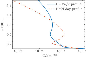
The parameter is an indicator of the strength of turbulence at a given location. In fact, it varies from place to place, throughout the day, and throughout the year. Several models have been developed. In this paper, the Hufnagel–Valley5/7 (H–V5/7) profile and Hefei-day profile are used, which are shown in Fig. 3.

The H–V5/7 profile is given by[12]

where w represents wind speed and A is the strength of the turbulence at the ground. Common values for these parameters are w = 21 m/s and A = 1.7 × 10⁻¹⁴ m−2/3.

The Hefei-day profile is the observational results of the atmospheric structure parameter in Hefei (China), which is defined by[13]

Fig. 3. Atmospheric turbulence profile models of H–V5/7 and Hefei-day.
3.2. Calculating the positions of phase screens

In this section, numerical calculations are carried out for the positions of phase screens and boundaries of each layer of atmosphere under H–V5/7 and Hefei-day profile. In the process of calculations, we use the ground H0 = 0, the propagation distance L = 10 km, the upper limit HN = L, and number of layers N = 1,2,3,…,7.

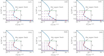
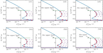
Figures 4(a1)4(a3) illustrate an example of positions of phase screen with the different layers (5, 6, and 7 layers) of atmosphere for the H–V5/7 profile. We can see that the positions of phase screen are not evenly distributed. Comparing the scheme of uniformly distributed phase screen, shown in Figs. 4(b1)4(b3), we can find that there is only one phase screen at most until the atmosphere is divided into seven layers in the specific observation area (mauve zone). By contrast, figures 4(a1)4(a3) show that two phase screens are distributed in similar area, which can adequately describe the effects of atmospheric turbulence near ground. The rest of phase screen has a more suitable position distribution in Figs. 4(a1)4(a3) instead of the dense distribution. Consequently, the positions of phase screen calculated by the iterative algorithm fit well with the atmospheric turbulence profile rather than mechanically placed phase screens at equal distance.

Similarly, figure 5 shows an example of positions of phase screen with the different layers (5, 6, and 7 layers) of atmosphere under the Hefei-day profile. Compared with the uniform distribution of phase screen, the results of the iterative algorithm also indicate that two phase screens are placed in the specific observation area (mauve zone). Combining the results under the H–V5/7 and Hefei-day profile, it can be seen that the above-mentioned iterative algorithm can be well applied in different atmospheric turbulence profile.

Tables 1 and 2 show the thickness of each layer and positions of phase screens for these two profiles. It can be seen that the position of phase screen in the first layer is gradually close to the ground with the increase of the number of layers. Similarly, the position of phase screen in the last layer gets closer to the upper limit of the turbulence profile.

Fig. 4. The positions of phase screen with the different layers (5, 6, and 7 layer) of atmosphere under the H–V5/7 profile (blue solid line). (a1)–(a3) The positions of phase screen (red circles) are calculated by the iterative algorithm. (b1)–(b3) The phase screens (red triangles) are evenly distributed. The dotted lines are base lines. The mauve zone is a specific observation area (its height is 1 km).
Fig. 5. The positions of phase screen (red triangles) with the different layers (5, 6, and 7 layers) of atmosphere under the Hefei-day profile (blue solid line). (a1)–(a3) The positions of phase screen are calculated by the iterative algorithm. (b1)–(b3) The phase screens are evenly distributed. The mauve zone is a specific observation area (its height is 1 km).
Table 1.

The thickness of each layer and positions of phase screens (PS) for the H–V5/7 profile.

.
Table 2.

The thickness of each layer and positions of phase screens (PS) for the Hefei-day profile.

.
3.3. Error analysis before and after optimization

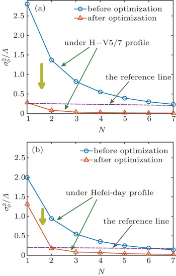
According to Eq. (13), we can obtain the relationship between the variance of residual phase error and the number of layers N. The wave number k and zenith angle θ can be regarded as a constant in a specific application. So the value of Λ(Λ = 2.91k2|θ|5/3) is also seen as a constant. Instead of calculating the values of directly, we only need to discuss the relationship between and N under the H–V5/7 profile and Hefei-day profile, shown in Fig. 6.

It can be seen that apparently decrease when the iterative optimization algorithm is used. Meanwhile, the decline rate of is highest particularly when the atmosphere is divided into two layers. As the number of layer increases, the values of tends to be stable. The improvement of the accuracy of multi-layered model of phase screen is limited with the increase of number of layers N. This means a defect that the large number of layers would greatly increase the amount of computation in numerical simulation, and it will also increase the experimental funding, since additional experimental device is required to simulate the layered atmosphere.

Fig. 6. The variance versus the number of layers N before optimization (uniformly distributed phase screen) and after optimization by the iterative algorithm, under H–V5/7 profile (a) and Hefei-day profile (b).

To describe the total ratio of error reduction after the iterative optimization algorithm is applied, we define the weighted mean of error reduction τ

where ηi = i is the weight value (i = 1,2, …,N), is the discrete-sum of i, and is the single ratio of error reduction for the i-layer of atmosphere. Here and are the variance of residual phase error for the i-layer of atmosphere before and after optimization, respectively.

Table 3.

The single and total ratio of error reduction after optimization for the H–V5/7 profile.

.

As shown in Tables 3 and 4, and the total ratio of error reduction after optimization τ are calculated under H–V5/7 and Hefei-day profile. We can see that was obviously decreased after the iterative optimization algorithm is used. Although the atmospheric turbulence profile is different, the iterative optimization algorithm can also improve the accuracy of multi-layered model of phase screen.

Table 4.

The single and total ratio of error reduction after optimization for the Hefei-day profile.

.
3.4. Analysis of the minimum condition

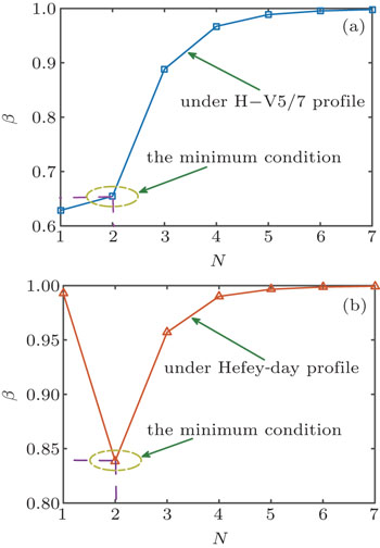
The minimum condition means that a least number of equivalent layers is required to obtain enough accuracy of multi-layered model of phase screen in the laboratory. In order to find out the minimum condition through the difference between the lines before and after optimization in Fig. 6, the similarity degree of these two curves is defined as

where xi = (5n,α γi), yi = (5n,α κi), γi is the values of before optimizing, κi is the values of after optimizing, α is a scaling factor, and n = 1,2,…,7. Here, we set α = ×10−7 to ensure the same sacle of xi(1) and xi(2), and yi(1) and yi(2) is also needed to be guaranteed for the same sacle.

The smaller the values of the similarity degree β is, the larger deviation between γi and κi is. Figure 7 shows a direct relationship between β and number of layers N under the H–V5/7 profile and Hefei-day profile. Obviously, the value of β increases as the value of N increases in Fig. 7(a). The value of β is very close when N is equal to one and two. However, the values of β is large when N is equal to one in Fig. 7(b). The rest of the value of β still increases with the value of N. So the value of β is relatively minimal on the whole when N is equal to two. Furthermore, it can be noticed that when N is equal to two, the values of is very small in Fig. 6, which is below the reference line. This means the largest decrease of , which indicates that the accuracy of multi-layered model of phase screen is improved most significantly at two layers.

Fig. 7. The similarity degree β versus number of layers N under H–V5/7 profile (a) and Hefei-day profile (b).
4. Conclusion

The iterative optimization algorithm of phase screen position along an inhomogeneous turbulent path has been discussed. For the H–V5/7 and Hefei-day profile, our results give the values of specific locations of phase screens, which can be used in a specific experiment. It is important to note that this iterative optimization algorithm is not limited by a certain turbulence profile. Compared with the uniform distribution of phase screens, the positions of phase screen calculated by the iterative algorithm can fit well with the specific turbulence profile. The variance of residual phase error was obviously decreased after the iterative optimization algorithm is used. The total ratio of error reduction after optimization is about 22.1 and 5.51 respectively for H–V5/7 and Hefei-day profile. Moreover, the minimum condition that the number of layers N is equal to two is also analyzed. When the scheme of this condition is used, the similarity degree of the curve before and after optimization is minimal.

Reference
1Puryear A LChan V W S2009Proc. SPIE746474640J
2Jin X L2010Acta Phys. Sin.59692(in Chinese)
3Liu Y Y Q BZhang W X2012Acta Phys. Sin.61124201(in Chinese)
4Coles W AFilice J PFrehlich R GYadlowsky M 1995 Appl. Opt. 34 2089
5Frehlich R 2000 Appl. Opt. 39 393
6Liu X YQian X MLi Y JRao R Z2012Chin. Phys. B23104203
7Schmidt J D2006Free-Space Optical Communications Performance Enhancement by Use of a Single Adaptive Optics Correcting Element (Ph.D. Dissertation)DaytonUniversity of Dayton
8Phillips J D2005Atmospheric Turbulence Simulation Using Liquid Crystal Spatial Light Modulators (MS Dissertation)DaytonAir Force Institute of Technology
9Qian X MZhu W YRao R Z2009Acta Phys. Sin.586633(in Chinese)
10Fusco TConan J MMichau VMugnier L MRousset G 1999 Opt. Lett. 24 1472
11Wallner E P 1994 Proc. SPIE 2201 110
12Parenti R RSasiela R J 1994 J. Opt. Soc. Am. 11 288
13Weng N QZong Z YXiao L MMa C SGong Z B1999High Power Laser and Particle Beams11673(in Chinese)