Anomalous transport in fluid field with random waiting time depending on the preceding jump length
Zhang Hong†, , Li Guo-Hua‡,
Department of Mathematics Teaching, Chengdu University of Technology, Chengdu 610059, China


† Corresponding author. E-mail: math_126@126.com

‡ Corresponding author. E-mail: ligh_0906@126.com

Project supported by the Foundation for Young Key Teachers of Chengdu University of Technology, China (Grant No. KYGG201414) and the Opening Foundation of Geomathematics Key Laboratory of Sichuan Province, China (Grant No. scsxdz2013009).

Abstract
Abstract

Anomalous (or non-Fickian) transport behaviors of particles have been widely observed in complex porous media. To capture the energy-dependent characteristics of non-Fickian transport of a particle in flow fields, in the present paper a generalized continuous time random walk model whose waiting time probability distribution depends on the preceding jump length is introduced, and the corresponding master equation in Fourier–Laplace space for the distribution of particles is derived. As examples, two generalized advection-dispersion equations for Gaussian distribution and lévy flight with the probability density function of waiting time being quadratic dependent on the preceding jump length are obtained by applying the derived master equation.

1. Introduction

The most popular model for describing the behavior of particle transport in fluid fields is the advection-dispersion equation (ADE) based on Fick’s diffusion law in hydrology and related sciences.[16] However, in recent years many tracer tests in natural complex porous media exhibit anomalous dispersion behavior deviating from Fickian diffusion, and the classical ADE is no longer suitable for describing this kind of tracer transport.[710]

One of the effective ways to quantify anomalous (or non-Fickian) transport in nonhomogeneous porous media is the continuous time random walks (CTRW’s) model.[1116] Based on various CTRW’s scholars obtain several generalization types of ADE, which can be used to describe the evolution of the probability density function (PDF) of the particles undergoing anomalous dispersion in flow fields.[17,18] Note that an assumption in the used CTRW models is that the energy of the non-Fickian particles does not have a direct effect on their transport behaviors. But in fact, the random sojourn times of the anomalous particles under certain circumstances maybe depend on their energy.

In 2006, Zaburdaev proposed a CTRW model in which the waiting time is connected with the preceding jump length. This model describes the dependence of the random waiting time on the energy and suggests a method that includes the details of the microscopic distribution over the waiting times and arrival distances at a given point.[19] Note that this generalized model has not been associated with the external velocity for the walking particle. As we know, to capture the behaviors of particle transport in moving fluids, the affect of convection velocity should be further considered.[17,20] One of the main aims of the present paper is to develop the CTRW model introduced by Zaburdaev coupling with a nonhomogeneous velocity field. Our generalized CTRW model can describe the behavior of the energy-dependence of random waiting time, and represent the influence of the velocity field on anomalous dispersion. In addition, we derive the corresponding master equation in the Fourier–Laplace domain from which the generalized ADE can be obtained in the macroscopic limit. As examples, we shall apply the new master equation to derive two generalized ADE’s for Gaussian distribution and lévy flight in linear flows when the microscopic distribution of the random sojourn time is quadratic dependent on the preceding jump length.

2. Classical CTRW model

For the generalization to anomalous transport in a fluid field, we first give the classical decoupled memory CTRW model in the one-dimensional case.[17,2025] In this scheme, the particle jumps from x to x + y with jump length PDF λ(y), and the waiting time before the particle makes two consecutive jumps has PDF ψ(t). The jump length and the waiting time are assumed to be independent random variables. The decoupled joint probability density obeys ψ(x,t) = λ(x)ψ(t). If ρ(x,t) is the PDF of the particle being in point x at time t and is the survival PDF, then

from which one obtains the well-known Montroll–Weiss equation

which can solve the problem of CTRW. Here, ρ0(k) represents the Fourier xk transform of the initial condition ρ0(x), ψ(u) denotes the Laplace tu transform of ψ(t), and ρ(k,u),ψ(k,u) are the Fourier–Laplace transform of ρ(x,t) and ψ(x,t).

3. CTRW model with random waiting time depending on the preceding jump length

Now, we recall the CTRW model with waiting time depending on the spent energy or the preceding jump length proposed by Zaburdaev.[19] In this model, each step of the particle requires some energy, and after making a jump a particle needs time to recover. The longer the preceding jump distance is, the longer the recovery and the waiting time are. It means that the PDF of the waiting time ψ(|y|,t) before making the second step depends both on the length of the preceding jump |y| and the waiting time t. Thus, the particle jumps from xy to x with the jump length PDF λ(y), and then waits at x for time t drawn from ψ(|y|,t), after which the process is renewed. By assuming that in the initial state all particles have zero arrival distances and zero resting times, one obtained the balance equation for the PDF ρ(x,t) of the particles

Here, j(x,t) is the escape rate, and satisfies the equation

where the survival time distribution depends both on the waiting time and the preceding jump length, the term Ψ0(t)ρ0(x) = Ψ(|0|,t)ρ(x,0) is supposed as the influence of the initial distribution, and ψ0(t) = ψ(|0|,t) is the waiting time PDF for the initial position. In Fourier–Laplace space, the PDF ρ(x,t) obeys the master equation for the CTRW model with waiting time depending on the preceding jump length

where the symbol ψ0(u) is the Laplace transform of ψ0(t), and Ψ0(u)ρ0(k), {Ψ(|x|,u)λ(x)}k, {ψ(|x|,u)λ(x)}k denote the Fourier–Laplace transform of Ψ0(t)ρ0(x), Ψ(|x|,t)λ(x), ψ(|x|,t)λ(x), respectively.

4. CTRW model in fluid fields with random waiting time depending on the preceding jump length

We shall now propose the energy-dependent random walk model in a moving fluid with an inhomogeneous velocity field v(x). As was shown in Refs. [17] and [20], in the Galilei variant model the jump length y for the moving particle dragged along the velocity v(x) is replaced by yτav(x), where τa represents an advection time scale, and τav(x) is the mean drag experienced by a particle jumping from the point x. In our model, we can introduce the PDF ϕ(y,t;x) of a length of step y with waiting time t which will depend on the velocity v(x) of the fluid with the starting point x of the jump, i.e.,

When v(x) = 0, the PDF ϕ(y,t;x) recovers the coupled density λ(y)Ψ(|y|,t) for the particle in Ref. [19]. Let ρ(x,t) be the PDF of the particle being in point x at time t and j(x,t) be the escape rate. By assuming that in the initial distribution all particles have zero arrival distances and zero resting times, we can find the balance equation for particles in a given point

By the relation equation (6), the above equation can be changed to the equivalent form

Fourier transforming xk and Laplace transforming tu of Eq. (8), we obtain

In the above expression j(k,u) is the Fourier–Laplace transform of j(x,t), and ϕ(k,u;kk′) represents the Fourier–Laplace transform of ϕ(x,t;x′) where from Eq. (6) and the fact that 𝓕(xf(x)) = i∂ f(k)/∂k one has

where the term Ψ(i/∂k,u)λ(k) represents the Fourier–Laplace transform of Ψ(|x|,t)λ(x).

To obtain the equation with respect to ρ(x,t) we then consider

By introducing

and applying the transform (x,t) → (k,u) of Eq. (11), we find

where

is the Fourier–Laplace transform of η(x,t;x′).

We now consider a linear velocity field, namely, v(x) = ωx, where ω is a constant. Then equation (12) becomes

where the symbol vk = τaωk.

In the limit τa → 0, equation (13) gives

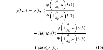
The above equation is a representation for j(k,u). To find the equation with respect to ρ(k,u), we express j(k,u) in terms of ρ(k,u) by using Eqs. (9) and (12)

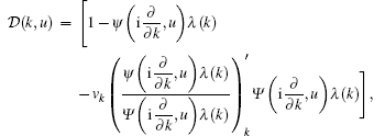
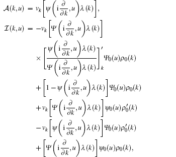
We substitute Eq. (15) into Eq. (14) and finally obtain the generalized master equation in Fourier–Laplace space for ρ(k,u) as

where

where the term 𝛪(k,u) denotes the influence of the initial condition. From Eq. (16), the corresponding advection-dispersion equation with the waiting time depending on the preceding jump length in velocity field v(x) = ωx can be derived by carrying out the macroscopic limit and inverting the Fourier–Laplace transform.

Remark 1 When the flow velocity v(x) = 0, equation (16) reduces to Eq. (5) derived by Zaburdaev.

Remark 2 If the waiting time PDF ψ(|y|,t) is independent of the preceding jump length and the initial condition is defined as ρ0(x) = δ(x), then equation (16) recovers the following master equation:

for the CTRW on linear moving fluids in a one-dimensional lattice obtained by Compte in Ref. [20].

Remark 3 For τa → 0, equation (9) gives

Substituting Eq. (15) into Eq. (18), we can also find Eq. (16).

5. Examples and generalized ADE’s

We shall apply the generalized master equation (16) to derive two generalized ADE’s for the particular cases when the jump lengths obey a Gaussian distribution or lévy flight and the waiting time PDF is quadratic dependent on the preceding jump length, i.e.,

where the length-dependent parameter α > 0.

We first consider the case for Gaussian jump length PDF

Then, the corresponding Laplace and Fourier transforms of ψ(|y|,t), λ(y) become

from which we find

Assuming ρ0(x) = δ(x), substituting Eqs. (23) and (24) and the initial condition ψ0(u) = 1, Ψ0(u) = 0 into Eq. (16), in the limit of τa → 0 and σ → 0 we obtain

with the finite value of A = τa/σ2.

Inverting Eq. (25) to the space-time domain kx and st, we then get a generalized ADE for the energy dependent random walks model in linear flows:

with the initial condition ρ0(x) = δ(x).

One can see that in the above generalized ADE both advection and diffusion coefficients depend on the length-dependent parameter α.

Secondly, we choose a Lévy distribution for the jump length, i.e.,

with 1 < β ≤ 2. Thus, for the length-dependent waiting time PDF

we have

For the initial condition ρ0(x) = δ(x), in the limit of small τa and σ, equation (16) then becomes

where A = limτa→0,σ→0(τa/σβ) is kept finite. The inverse Fourier–Laplace transform of Eq. (30) leads to the generalized fractional ADE:

with the initial condition ρ0(x) = δ(x). Here, the operator , is the fractional derivative of the Riemann–Liouville type,[26,27] equal in Fourier xk space to (ik)3−β. It should be noted that in Eq. (31) the advection and diffusion coefficients both involve the length-dependent parameter α. Note also that this generalized fractional equation (31) reduces to Eq. (26) when β = 2.

6. Conclusions

The derivation of ADE led to wide applications for particle transport in flow fields. In recent years, several authors have begun to study the generalizations of ADE’s based on various CTRW’s. In this paper, we developed a rather general continuous time random walk model in moving fluids with the waiting time depending on the preceding jump length or the energy, and derived the generalized master equation (16) for this new random walk model. Moreover, by using Eq. (16), we obtained two generalized ADE’s for Gaussian distribution and lévy flight with the waiting time PDF being quadratic dependent on the preceding jump length, and showed that in the generalized ADE’s both advection and diffusion coefficients involve the length-dependent parameter. There are problems such as that the continuous time random walk model in moving fluids whose waiting time depends on the time varying energy and the corresponding generalized master equation are still unknown.

Reference
1BradleyD NTuckerG EBensonD A 2010 J. Geophys. Res. 115 F00A09
2SchumerRMeerschaertM MBaeumerB 2009 J. Geophys. Res. 114 F00A07
3Benson D AWheatcraft S WMeerschaert M M 2000 Water Resour. Res. 36 1403
4LiuG JGuoZ LShiB C 2016 Acta Phys. Sin. 65 014702 (in Chinese)
5BerkowitzBCortisADentzMScherH 2006 Rev. Geophys. 44 RG2003
6Chang F XChen JHuang W2005Acta Phys. Sin.541113(in Chinese)
7Zhang YMartin R LChen DBaeumer BSun H GLi C 2014 J. Geophys. Res. Earth Surf. 119 2711
8Baeumer BBenson D AMeerschaert M MWheatcraft S W 2001 Water Resour. Res. 37 1543
9Addison P SQu BNdumu A SPyrah I C 1998 Math. Geol. 30 695
10Atangana A 2014 J. Earth Syst. Sci. 123 101
11Fourar MRadilla G 2009 Transp. Porous. Med. 80 561
12Wang JZhou JLv L JQiu W YRen F Y 2014 J. Stat. Phys. 156 1111
13Zhang HLi G HLuo M K 2013 J. Stat. Phys. 152 1194
14Shahmohammadi-Kalalagh SBeyrami H 2015 Geotech. Geol. Eng. 33 1511
15 YBao J D 2011 Phys. Rev. 84 051108
16Zhang HLi G HLuo M K 2012 Chin. Phys. 21 060201
17Metzler RKlafter J 2000 Phys. Rep. 339 1
18Baeumer BBenson D AMeerschaert M M 2005 Physica 350 245
19Zaburdaev V Y 2006 J. Stat. Phys. 123 871
20Compte A 1997 Phys. Rev. 55 6821
21Liu JYang BChen X SBao J D 2015 Eur. Phys. 88 88
22Emmanuel SBerkowitz B 2007 Transp. Porous. Med. 67 413
23Bakunin O G2008Turbulence and Diffusion: Scaling Versus EquationsBerlinSpringer-Verlag223226223–6
24Klafter JSilbey R 1980 Phys. Rev. Lett. 44 55
25Gorenflo RVivoli AMainardi F 2004 Nonlinear Dyn. 38 101
26Podlubny I1999Fractional Differential EquationsSan DiegoAcademic Press627762–77
27Li G HZhang HLuo M K 2012 Chin. Phys. 21 128901