† Corresponding author. E-mail:
Project supported by the National Natural Science Foundation of China (Grant Nos. 41230421 and 41605075) and the National Basic Research Program of China (Grant No. 2013CB430101).
The present work reports the development of nonlinear time series prediction method of genetic algorithm (GA) with singular spectrum analysis (SSA) for forecasting the surface wind of a point station in the South China Sea (SCS) with scatterometer observations. Before the nonlinear technique GA is used for forecasting the time series of surface wind, the SSA is applied to reduce the noise. The surface wind speed and surface wind components from scatterometer observations at three locations in the SCS have been used to develop and test the technique. The predictions have been compared with persistence forecasts in terms of root mean square error. The predicted surface wind with GA and SSA made up to four days (longer for some point station) in advance have been found to be significantly superior to those made by persistence model. This method can serve as a cost-effective alternate prediction technique for forecasting surface wind of a point station in the SCS basin.
Surface wind is an important ocean parameter. Forecasting ocean surface wind involves two aspects: the wind speed and wind direction, and the zonal and meridional wind components. Prediction of surface wind speed is very important in many applications, such as planning, construction, and operation-related works in the oceanic areas, and so on. Meanwhile, prediction of the surface wind components constitutes an important component of ocean state prediction using numerical ocean and atmospheric models.[1]
Predictability of the ocean surface wind including wind speed and wind components has achieved considerable success using numerical models in many studies.[1,2] However, the numerical prediction models suffer from various drawbacks, such as incomplete physics, incorrect initial conditions, etc. In particular, when point forecasts at specific locations are required, the numerical prediction models are disadvantageous because there are always extremely complex and are highly computer intensive due to the huge amount of input information, such as the vertical profiles of humidity, temperature, and so on.[3,4]
It is thus interesting to explore the possibility of predicting the surface wind using only past observations without the need for sophisticated numerical models. Over the years, various such data-adaptive approaches, such as linear regression, support vector machines,[5] artificial neural networks (ANNs),[6] genetic algorithm (GA),[7] and so on,[8,9] have been proposed for prediction of the nonlinear data series. The GA algorithm, which is based on Darwin’s evolutionary theory,[7,10,11] is a modern and powerful nonlinear data fitting algorithm. One of the advantages of GA algorithm is that it does not require very long time series of wind observations. Another advantage is that it provides an explicit analytical forecast equation.[12]
The predictive skill of GA has been demonstrated in the cases of sea surface temperature (SST) in the Alboran Sea,[13] summer rainfall over India,[14] SST and sea level anomaly in the Ligurian Sea,[15] wave heights in the north Indian Ocean (NIO),[3,4] the tidal currents in the Arabian Sea,[16] and so on. Meanwhile, ocean surface wind prediction with in situ and scatterometer observations using GA have been tested in the NIO and the results show that predictions with GA made up to three days have been found to be quite encouraging.[3] Due to the specific characteristic of the GA algorithm, the prediction models for different point stations and different basins are different.[3,4]
In the present study, the GA technique has been used to forecast the surface wind in the South China Sea (SCS), which is an important ocean due to the high level of scientific and economic interests in the area. In a previous diagnostic study, Basu et al.[3] explored the ability of predicting the surface wind in the NIO. Apart from the different basin, another novel feature of the present study is the use of singular spectrum analysis (SSA) for noise reduction, which is not tested in previous study. It is known that the GA algorithm, in principle, can predict a strictly deterministic, albeit chaotic, and time series. However, the inevitable presence of noise in any physical system and observations introduces spurious features, not amenable to prediction.[16] Hence, a pre-filtering of the data series using a noise reduction technique becomes absolutely necessary. The SSA is arguably the best known data adaptive approach for noise reduction.[1]
Descriptions of the GA algorithm for prediction and SSA for noise reduction are provided in Sections 2 and 3 separately. Section 4 gives the detail of the used scatterometer observations. The results of the GA algorithm compared with the persistence model for forecasting surface wind speed and surface wind components in the SCS are given in Section 5. Section 6 is the conclusion and discussion.
The GA algorithm which is based on the Taken’s theorem has been described in detail by earlier works.[3,10]
Briefly, given a deterministic time series {x(ti)},i = 1,…,N, there exists a smooth map β :

The GA algorithm approximates the mapping β using a technique borrowed from evolutionary biology. The algorithm starts with an initial population of N “equation strings”, and includes the following major steps: (1) initialization, (2) computing the fitness, (3) ranking the agents, (4) choosing the mates, (5) reproduction and crossover, and (6) mutation. The detailed description of the algorithm can be found in Ref. [3]. The fitness for the equation string gj which is necessary for step (2) can be computed as


Because of the measurement errors, the scatterometer observations are inevitably a mixture of deterministic part as well as random part. Hence, it is absolutely necessary to reduce the noise before carrying out a GA forecast. The SSA is arguably the best known data adaptive approach for noise reduction, and hence has been adopted in the present study for reducing noise. The SSA was described in detail and used in Ref. [10]. This happened because Takens’s theorem, which is the theoretical basis of GA, can only be applied in the absence of noise and an obvious presence of noise in any physical measurement will induce inappropriate reconstructions.
Briefly, for the time series of observations denoted by A, one has to form a trajectory matrix
In this paper, the time series of daily averaged wind speed (calculated from wind components) and wind components (including zonal and meridional) measured by the scatterometer onboard QuikSCAT satellite at three selected locations in the SCS are used. A scatterometer, which can provide all-day and large-scale wind field information, has become a main instrument to obtain surface wind field.[17,18] The scatterometer wind used in this paper is distributed by the French Research Institute for Exploitation of the Sea (IFREMER). The wind has been compared with daily, weekly, and monthly averaged forecasts of the European Centre for Medium range Weather Forecast (ECMWF) model, which shows that the average features are well captured over the global oceans. In addition, comparison with the daily averaged Tropical Atmosphere/Ocean (TAO) and the National Data Buoy Center (NDBC) buoy data at Pacific and Atlantic Oceans show small root-mean-square difference.[3] The wind speed prediction is particularly important for marine works, such as ship planning, construction, and so on, whereas the zonal and meridional wind components are necessary for forecasting the sea state with numerical models. Hence, the wind speed and wind components measured by scatterometer have been chosen in order to show that the algorithm performs equally well for both wind-type predictions.
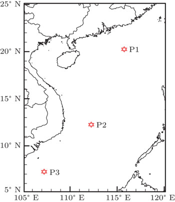
Three locations in the SCS of QuikSCAT scatterometer observations (Station P1 at (20.25° N, 115.75° E), P2 at (12.25° N, 112.25° E), and the location (7.25° N, 107.25° E) for P3) have been used in order to demonstrate the performance of the algorithm in any particular basin of the SCS. The location details and observation duration of the winds are provided in Table
| Table 1. Location details and observation duration of remotely sensed scatterometer winds. . |
First, the SSA was applied to the WTS (WT stands for the time series of wind speed or wind components) of different point stations using a window size of 370. Then, the GA was applied to predict the filtered time series of the WTS and the fluctuation part (deviation of the filtered WT from the actual WT). The forecast winds were reconstructed with the predicted WTS (including the predicted filtered WTS and the predicted fluctuation part) and compared with the actual winds for evaluating the quality of forecast.
The following parameters were used to train the GA algorithm: the number of equation strings was 60, the total number of arguments and operators allowed was 20 in all the cases, the embedding dimension varied from 4 to as high as 25, and the best embedding dimension m was estimated by trial and error in the present study. The mutation rate was chosen to be 0.01. Finally, the number of iterations required to achieve maximum strength index also varied from case to case and the maximum number was 5000.
Due to the unknown real wind in the previous research,[3] it is instructive to compare the GA forecast with the forecast carried out by a persistence model. For a given WT, the persistence model is defined by the following equation:

The first 2960 points of the wind time series were used to train the algorithm and the remaining points were used for validation.
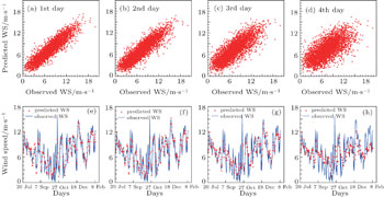
The scatter plots of the wind speed predicted by the GA versus the actual wind speed at P2 point location, and some part of the corresponding time series at the same location are shown in Fig.
Meanwhile, for the 1-day to 4-day forecast, the GA prediction is much better than the persistence model forecast, which is true for the wind speed prediction of all the three points, as shown in Table
Although the coefficient of determination R2 (square of the coefficient of correlation) between the observations and predictions is very similar for the three points, the RMSE of wind speed for P1 point is worse than P2 and P3 points (Table
| Table 2. Comparison of predicted wind speed by GA and persistence model at the three locations. The RMSE means root mean square error of forecast in meters/second. R2 is shown only for the case of GA. . |
The equations for 1-day forecast of wind speed at P2 station are provided in Appendix A.
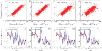
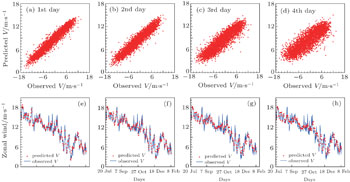
The GA algorithm and persistence model are also used to forecast the zonal and meridional wind components with scatterometer observations. In Fig.
In Table
| Table 3. Comparison of predicted zonal and meridional wind components by GA and persistence model at the three locations. . |
Meanwhile, as shown in Table
The equations for 1-day forecast of wind zonal and meridional components at P2 station are also given in Appendix A.
Apart from persistence model prediction, one can also use an autoregressive model approach, which is a classical approach for time series modeling. However, the autoregressive approach is a linear approach and has been proven to be unable to improve upon the persistence prediction quite significantly for wind prediction in the Bay of Bengal BOB.[3] Hence, it is not necessary to compare the GA algorithm with the autoregressive approach in the present work.
In the present work, a technique known by the name of GA with SSA has been used to predict surface wind (including wind speed and wind components) in the SCS with scatterometer observations. Since the technique can in principle be used to predict a strictly deterministic time series, whereas the time series of scatterometer wind (WT) inevitable has noise, SSA has been applied to reduce the noise. Then, the GA has been carried out to predict the time series of the WTs (including the filtered WTs and the fluctuation part from SSA).
The GA technique has been used to carry out 1 to 4 days ahead forecast of wind speed and wind components for three points with scatterometer observations in the SCS basin. The forecast has been compared with persistence model forecast and it has been found that GA algorithm is able to significantly improve upon the persistence model forecast with leading times of 1 to 4 days in the SCS basin for both wind speed and wind components prediction. Meanwhile, the predictability for different station in the basin is different, for example, the P1 station that is influenced by Taiwan strait has less predictability, and the improvement of GA algorithm also shows large differences for different station. It can be concluded that the algorithm yields an encouraging performance and has the potential to be used by an operational agency which is interested in the ocean-state forecast of the SCS basin.
One should know that an important advantage of the GA algorithm is that it provides explicit analytical forecast equations for surface wind. Another added advantage is that much less input information is required by this algorithm compared with the sophisticated atmospheric models. In the future, this algorithm could be extended to wind field prediction and it will be tested with the scatterometer wind from the HY-2 satellite that was launched by China.
| 1 | |
| 2 | |
| 3 | |
| 4 | |
| 5 | |
| 6 | |
| 7 | |
| 8 | |
| 9 | |
| 10 | |
| 11 | |
| 12 | |
| 13 | |
| 14 | |
| 15 | |
| 16 | |
| 17 | |
| 18 |


