Since Feynman^[1,2] put forward the concept of quantum computer following the quantum mechanics laws in 1980s, researchers started to study theoretically and experimentally the quantum computer (QC), and QC gradually became a hot spot of information science. The basic information storage and process unit of QC is qubit. Many two-state quantum systems can be used as the carrier of qubit.^[3–6] People have proposed various solutions to obtain qubit. At present, the solutions which have made some progresses include the cavity quantum electrodynamics, the ion trap, the liquid-state nuclear magnetic resonance, etc.^[7–10] However, the common disadvantage of these solutions is unable to obtain a large number of qubits. To achieve the large scale integration of qubits, we have to adopt a solid-state qubit system. This system is easier to achieve miniaturization and integration of a large number of qubits, and it has more potential to manufacture a truly practical QC, thus, many researchers start to study the quantum dot qubit and have obtained a series of important results.^[11–14]

In recent years, many researchers studied the effect of the electron–phonon interaction on qubit in quantum dot.^[15–18] Most of those studies are limited to discuss the qubit structured by the monopolaron ground state and the first excited state, and there is no doubt that it is correct for the III–V semiconductor quantum dot. However, with the development of the semiconductor material growth technology, the I–VII semiconductors (such as RbCl, KI, etc.) have drawn much attention in recent years. As the electron–phonon coupling constant of the I–VII semiconductors is an order of magnitude larger than that of the III–V semiconductors, and the electron–phonon interaction in the quantum dot made of such materials becomes even stronger due to the lower dimensionality (usually the electron–phonon coupling strength is greater than 6), the bound state of bipolaron can be formed by the interaction between two identical electrons through the phonon field.^[19–21] In the study of bipolaron in magnetic field, one of the authors^[21] first proposed the concept of magneto-bipolaron. It is no doubt that, for the quantum dot made of I–VII semiconductor materials, it is impossible and not necessary to restrain the bipolaron formation, and the study of the bipolaron qubit has more practical significance and potential in application than the study of the polaron qubit alone. We adopt the variational method of the Pekar type based on the Lee–Low–Pines (LLP) unitary transformation and study the property of the qubit structured by the strong-coupling magneto-bipolaron ground state and the first excited state in the quantum dot under a magnetic field. We propose the conception of magneto-bipolaron qubit in the quantum dot made of I–VII semiconductors, complement and perfect the phonon effect of solid state quantum information.

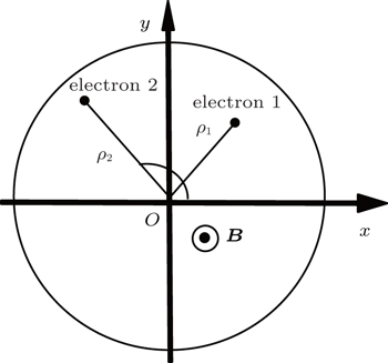
We consider a two-electron system which is restrained in a two-dimension (x–y plane) parabolic quantum dot and interacts with the longitudinal optical (LO) phonon. The external magnetic field B is along the z direction. The vector potential is A = B(−y,x,0) /2. We set the center of the quantum dot as origin point O to establish the plane polar coordinates, see Fig. 1. The system’s Frölich Hamiltonian^[20,21] can be written as

Fig. 1.

	Figure Option ViewDownloadNew Window
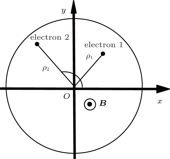
	Fig. 1. Schematic diagram of quantum dot.

To obtain the system energy, the extremum problem about the expectation value of the variational function U⁻¹ HU in the state |Ψ⟩ is discussed here. According to the variational principle,

To show the variations of E₀, E₁, Q, and T₀ with ω_c, ω₀, η, and α clearly and intuitively, the results of numerical calculations are shown in Figs. 2–7, taking ħω_LO as the unit of energy, ω_LO as the unit of ω₀ and ω_c, and r_p as the length unit.

Figure 2 shows the variations of the ground state energy E₀ and the first-excited state energy E₁ of magneto-bipolaron with (a) the confinement strength ω₀ at different electron–phonon coupling strength α and (b) the dielectric constant ratio η at different resonant frequency of the magnetic field ω_c. From Figs. 2(a) and 2(b), it can be seen that the ground state energy of magneto-bipolaron E₀ < 0, and the absolute value of E₀ is very large. This indicates that the ground state of magneto-bipolaron is a steady bound state and needs huge energy to excite it, so the first-excited state of magneto-bipolaron should be structured by one electron staying in the ground state and the other electron being excited to the first-excited state. This is why we use Eq. (6) as the ground state trial wave-function of magneto-bipolaron and Eq. (7) as the first-excited state trial wave-function. It can be seen from Fig. 2(a) that the absolute value of the ground state energy |E₀| decreases with increasing ω₀, while the first-excited state energy E₁ increases with increasing ω₀. |E₀| and E₁ increase with increasing α when ω₀ is fixed. It can be seen from Fig. 2(b) that |E₀| and E₁ increase with increasing η. When η is fixed, |E₀| decreases with increasing ω_c, but E₁ increases with increasing ω_c.

Fig. 2.

	Figure Option ViewDownloadNew Window
	Fig. 2. Variations of the ground state energy E0 and the first-excited state energy E1 of magneto-bipolaron with (a) the confinement strength ω0 at different electron–phonon coupling strength α and (b) the dielectric constant ratio η at different resonant frequency of the magnetic field ωc.

Figure 3 shows the variations of the oscillation period T₀ with (a) the confinement strength ω₀ at different electron–phonon coupling strength α and (b) the dielectric constant ratio η at different resonant frequency of the magnetic field ω_c. It can be seen from Fig. 3(a) that T₀ decreases with increasing ω₀ and α. This is because the energy difference ΔE = E₁ − E₀ increases with increasing ω₀ and α, which can be seen from Fig. 2(a). It can be seen from Fig. 3(b) that T₀ decreases with increasing η and ω_c. This is because the energy difference Δ E = E₁ − E₀ increases with increasing η and ω_c, which can be seen from Fig. 2(b). Here we can see that the magneto-bipolaron qubit coherence decreases with increasing confinement strength of the quantum dot, electron–phonon coupling strength, dielectric constant ratio, and external magnetic field. This is in agreement with the discussion in Refs. [15]–[18].

Fig. 3.

	Figure Option ViewDownloadNew Window
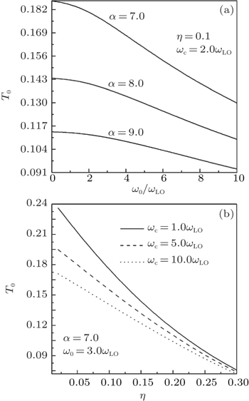
	Fig. 3. Variations of the oscillation period T0 with (a) the confinement strength ω0 at different electron–phonon coupling strength α and (b) the dielectric constant ratio η at different resonant frequency of the magnetic field ωc.

Figure 4 shows the variations of the probability density Q with (a) the confinement strength ω₀ and (b) the dielectric constant ratio η. It can be seen from Fig. 4(a) that Q first increases to a maximum and then quickly decreases to a minimum and finally increases again in a very short time. From Fig. 4(b), it is not difficult to see that Q increases oscillatory with increasing η.

Fig. 4.

	Figure Option ViewDownloadNew Window
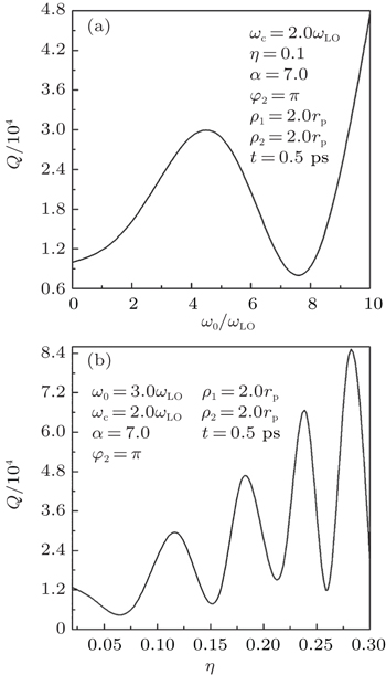
	Fig. 4. Variations of the probability density Q with (a) the confinement strength ω0 and (b) the dielectric constant ratio η.

Figure 5 shows the variations of the probability density Q with (a) polar angle φ₂ and (b) time t. From Fig. 5, it can be seen that Q oscillates periodically with increasing φ₂ or t.

Fig. 5.

	Figure Option ViewDownloadNew Window
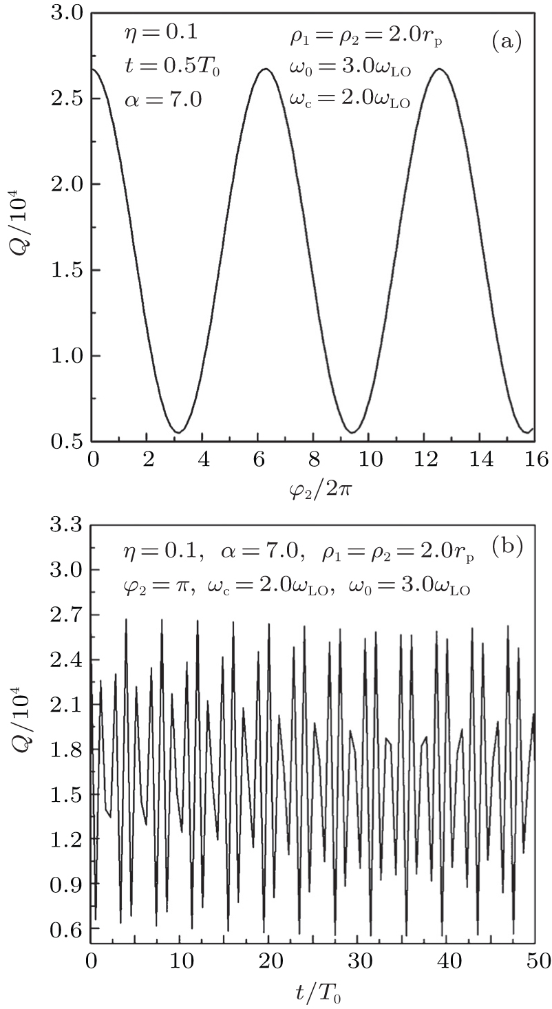
	Fig. 5. Variations of the probability density Q with (a) polar angle φ2 and (b) time t.

From Figs. 4 and 5, we can find that the probability density Q of the two electrons in the qubit oscillates periodically with increasing time t, angular coordinate φ₂, and dielectric constant ratio of the medium η. Physically, it is a representation of volatility of bipolaron superposition state. To be specific, the phase change of the probability wave of bipolaron depends on time t.

Figure 6 shows the variations of the probability density Q with coordinate ρ₁ at (a) different electron–phonon coupling strength α and (b) different resonant frequency of the magnetic field ω_c. From Fig. 6(a), it can be seen that Q quickly decreases with increasing ρ₁ and α has certain influence on the change of Q with ρ₁. From Fig. 6(b), it is not difficult to see that ω_c also has certain influence on the change of Q with ρ₁. From Fig. 6, we find that the probability of electron 1 appearing near the center of the quantum dot (ρ₁ < 6.0r_p) is larger, and the probability of appearing away from the center of the quantum dot is smaller.

Fig. 6.

	Figure Option ViewDownloadNew Window
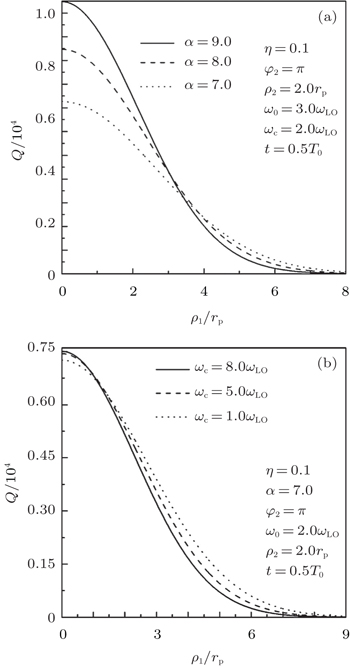
	Fig. 6. Variations of the probability density Q with coordinate ρ1 at (a) different electron–phonon coupling strength α and (b) different resonant frequency of the magnetic field ωc.

Figure 7 shows the variations of the probability density Q with coordinate ρ₂ at (a) different electron–phonon coupling strength α and (b) different resonant frequency of the magnetic field ω_c. From Fig. 7(a), it can be seen that Q first quickly decreases to a minimum and then slowly increases to a maximum and finally decreases slowly to zero. In the meantime, α has certain influence on the change of Q with ρ₂. From Fig. 7(b), it can be seen that the variations of Q with ρ₂ at different ω_c is very similar to those at different α in Fig. 7(a). From Fig. 7, we find that the probability of electron 2 appearing near the center of the quantum dot (ρ₂ < 3.0r_p) is larger, and the range of electron 2 is smaller than that of electron 1, and the probability of appearing away from the center of the quantum dot is smaller. Here we can see that the probability of electron appearing near the center of the quantum dot is larger. This is because the harmonic confinement potential of the quantum dot is smaller in the central area and the system energy is lower when the electrons are at the central area.

Fig. 7.

	Figure Option ViewDownloadNew Window
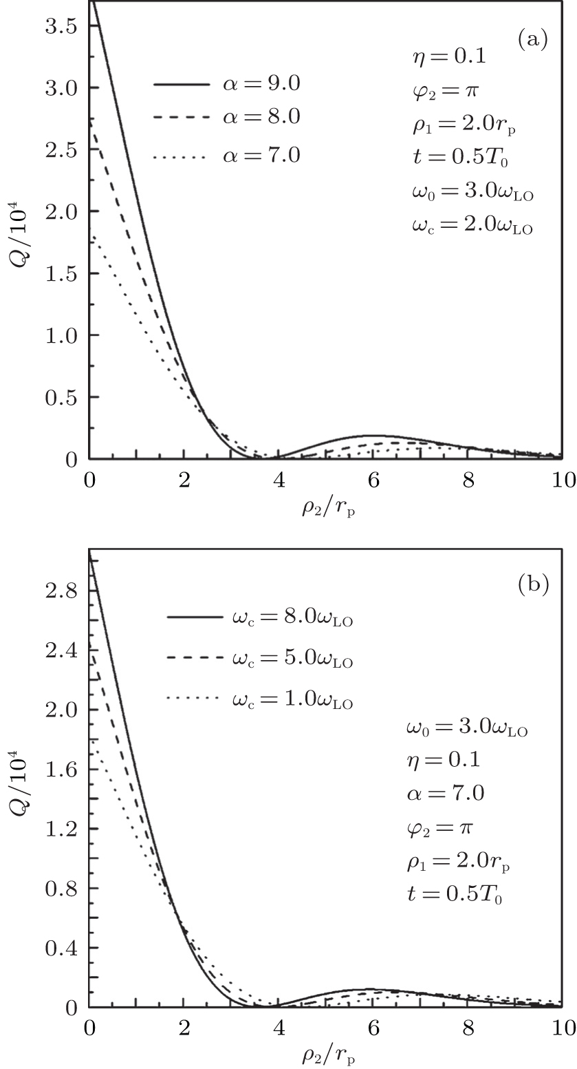
	Fig. 7. Variations of the probability density Q with coordinate ρ2 at (a) different electron–phonon coupling strength α and (b) different resonant frequency of the magnetic field ωc.

Based on the variational method of Pekar type, we study the energies and the wave-functions of the ground and the first-excited states of magneto-bipolaron, which is strongly coupled to the LO phonon in a parabolic potential quantum dot under an applied magnetic field, thus built up a quantum dot magneto-bipolaron qubit. The following results are obtained. (i) The oscillation period of the probability density of the two electrons in the qubit decreases with increasing electron–phonon coupling strength α, resonant frequency of the magnetic field ω_c, confinement strength of the quantum dot ω₀, and dielectric constant ratio of the medium η. (ii) The probability density of the two electrons in the qubit oscillates periodically with increasing time t, angular coordinate φ₂, and dielectric constant ratio of the medium η. (iii) The probability of electron appearing near the center of the quantum dot is larger, and the probability of electron appearing away from the center of the quantum dot is much smaller.