Cane sugar (sucrose) is a basic livelihood commodity produced from sugarcane. Among the major cane sugar producers and consumers, China ranks the 3rd, accounting for 7% of the world total. Within China, the Guangxi Autonomous Region in southwest China is the biggest producer of cane sugar in the country, accounting for more than 60% of the market. Unlike in developed countries such as USA and Australia, cane sugar production in most factories in Guangxi and many other regions in China has not been made automatic, partly due to a lack of understanding of the fundamental physics and chemistry involved in the production process.

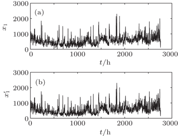
In general, cane sugar processing consists of six phases: milling, clarification, evaporation, crystallization, centrifuging, and drying so as to obtain white sugar, brown sugar, and other products.^[1] In particular, the juice from the milling workshop is called the mixed juice, which contains water, sucrose, bagasse, soil, sand, reduced sugar, and many organic and inorganic non-sugar components. The latter are residual nutrients in the sugarcane, including colloidal substances, inorganic salts (iron, magnesium, aluminum, calcium, and so on), and pigments. Affecting the appearance, color, and concentration of the sugar, the non-sugar components are detrimental to the sugar production, and thus should be carefully removed. This is the aim of the next stage, the clarification stage. It is characterized by two target variables: the color of the produced sugar and its clarity degree. A typical example of the temporal variation of these variables is shown in Fig. 1, where the time covered is the entire harvest season of sugarcane in Gaungxi, China, which is slightly less than 4 months. The long-range correlations in these time series are thought to hinder the automation of cane sugar production from sugarcanes, as long-range correlations mean that persistent deviations from the target values of these variables may last for a considerable period of time.^[1] The quality of clarification is characterized by the smallness in color value and the largeness in clarity degree.

Fig. 1.

	Figure Option ViewDownloadNew Window
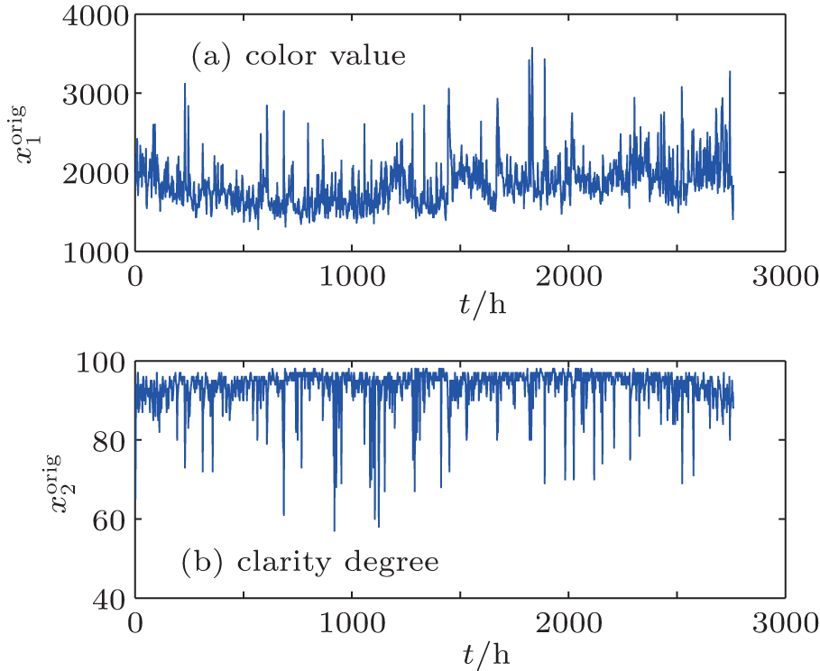	Fig. 1. Raw data of (a) color value and (b) clarity degree

There has been a great deal of effort expended to improve the clarification of the mixed juice by using physical and chemical means, including using enzymes to reduce viscosity,^[2] improving the flocculants,^[3] employing electrocoagulation,^[4] and enhancing decolorization by hydrodynamic cavitation.^[5] These approaches are hoped to directly or indirectly enhance the absorption of impurities by flocs and sediments in the settler. Unfortunately, the effectiveness of the methods has not been thoroughly validated. As a result, these methods have not been adopted in practice yet.

There also has been effort to use neural network based prediction schemes^[6,7] to improve cane sugar production. Being black or gray box-based approaches, however, they have not yielded much understanding of the basic physics and chemistry involved in the clarification process, and thus have not helped much with cane sugar production. Observing Fig. 1, we realize that there are two different ways to improve clarification. One is to drastically upgrade the facility in the cane sugar production factory such that the color value can be made significantly smaller while the clarity degree can be made significantly larger. This approach is costly and not realistic. The other approach is to mainly stick with the available facility, but to manage to make the variations in color and clarity degree as small as possible. In other words, the color value would always be close to the minimal value with the clarity degree close to the maximal value shown in Fig. 1. Albeit not as good as the first scenario, this approach is often more than sufficient, since the observed raw color value and clarity degree already conform to industrial standards. This is the scenario that we will focus on in this work. Specifically, we will use multiplicative cascade multifractal to understand whether the variations in the color value and the clarity degree are purely random, or have system-wide causes. If the latter is the case, then it is very likely that effective means can be devised to substantially improve the clarification of the mixed juice from the milling stage.

The multifractal is one of the most important models contributed by complexity science. It is worth noting with the excitement that there has been a great deal of research on complexity science by the Chinese physical community, including works on stochastic resonance, bifurcations, and chaos.^[8–22]

Mathematically, multifractals are characterized by many or infinitely many power-law relations. In this paper, we work with a specific type of multifractal, called the random multiplicative process model, to analyze the color value and the clarity degree. This type of multifractal was initially developed to understand the intermittent features of turbulence.^[23–25] Mandelbrot was among the first to introduce this concept. Parisi and Frisch's work^[26] on turbulence has made it widely known. It has been applied to the study of various phenomena, such as rainfall,^[27] liquid water distributions inside marine stratocumuli,^[28,29] finance,^[30] tropical deep convective variability,^[31] and network traffic.^[32,33]

The remainder of the paper is organized as follows. In Section 2, we perform a distribution analysis of the clarification process, to infer whether the variations in the color value and the clarity degree may have system-wide causes. In Section 3, we employ the cascade multiplicative multifractal process to model the variations in the color and clarity degree. We show that those variations can be characterized by multifractal processes. The concluding discussion is presented in Section 4.

As we have pointed out, in order to infer whether the variations in the color value and the clarity degree may have system-wide causes, we may focus on the variations in the color value and clarity degree around the minimal and the maximal values, respectively. Denote the raw data of the color value and clarity degree by and The scenario taken here amounts to studying

Fig. 2.

	Figure Option ViewDownloadNew Window
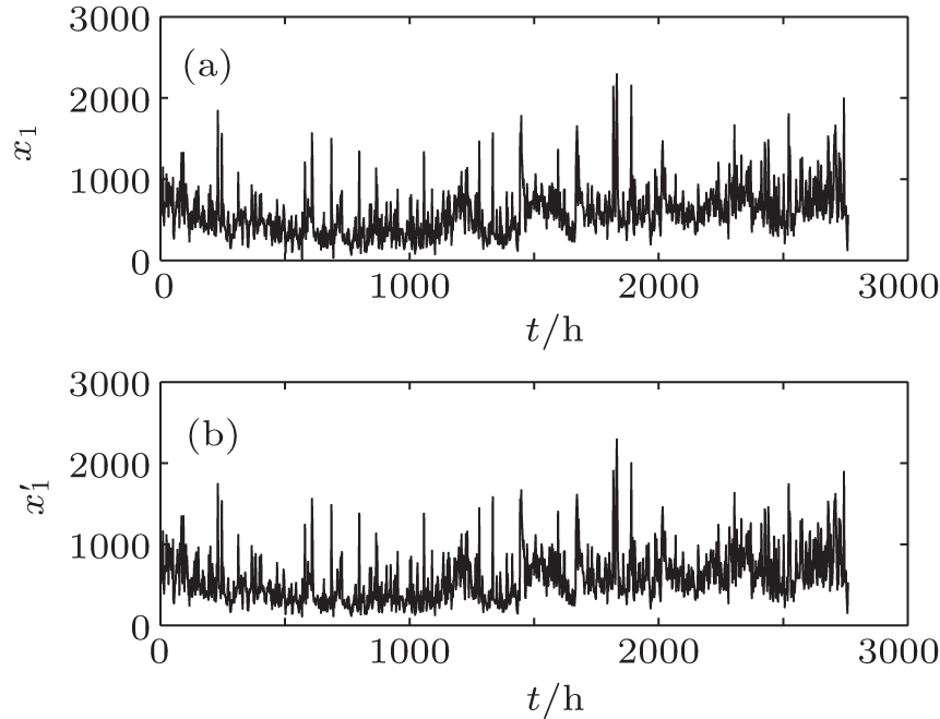	Fig. 2. Modeling of the variation of color value: (a) measured and (b) simulated with σ = 0.078.

Fig. 3.

	Figure Option ViewDownloadNew Window
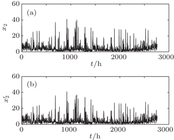
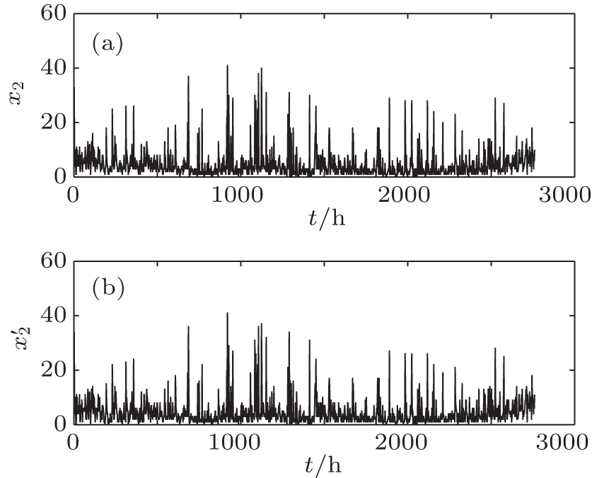	Fig. 3. Modeling of the variation of clarity degree: (a) measured and (b) simulated with σ = 0.1385.

Let us perform a distribution analysis of these variables. Concretely, we will check whether they may follow two specific distributions. One is an exponential distribution, which may be expressed by its probability density function (PDF)

We hypothesize that if the distribution is close to exponential, or other thin-tailed distributions, then the variations in the color value and the clarity degree are simply random and do not have system-wide causes. However, if the distribution is heavy-tailed, then the variations in the color value and the clarity degree may have system-wide causes.

We have estimated the distributions for the time series data of x₁ and x₂. The results are shown in Fig. 4. We observe that both have powerlaw-like distributions. However, the α parameter for the color value is quite large. As a result, the scaling for the powerlaw behavior is valid for a range less than one decade, as shown by the fitted straight line in Fig. 4(a). In contrast, the distribution in the clarity degree is heavy-tailed, with α < 2, and a scaling region close to one decade. These analyses suggest that the variations in the color value and the clarity degree may indeed have system-wide causes, and thus may be further analyzed by advanced methods.

Fig. 4.

	Figure Option ViewDownloadNew Window
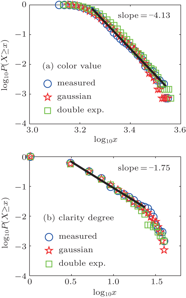	Fig. 4. Complementary cumulative density function (CCDF) for the measured and simulated data with multiplier distributions being Gaussian Eq. (8) and double-exponential Eq. (9). (a) Color value and (b) clarity degree.

To gain deeper insights into the clarification of sugarcanes, in this section we perform a multifractal analysis of x₁ and x₂.

With the framework of the cascade multiplicative model, one considers the moments

To better understand multifractal formalism, we consider below the random multiplicative cascade model. The conservative model, which is most pertinent here, is specified as follows. Consider a unit interval. Associate it with a unit mass. Divide the unit interval into two, say, left and right segments of equal length. Also, partition the associated mass into two fractions, r and 1 – r, and assign them to the left and right segments, respectively. The parameter r is in general a random variable, governed by a PDF P(r), 0 ≤ r ≤ 1. The fraction r is called the multiplier. Each new subinterval and its associated weight are further divided into two parts following the same rule. This procedure is schematically shown in Fig. 5, where the multiplier r is written as r_ij, with i indicating the stage number and j (assuming only odd numbers, leaving even numbers for 1 – r_ij) indicating the positions of a weight on that stage. Note that the scale (i.e., the interval length) associated with stage i is 2^–i. We assume that P(r) is symmetric about r = 1/2 and has successive moments μ₁, μ₂, …. Hence r_ij and 1 – r_ij both have marginal distribution P(r). The weights at the stage N, {w_n, n = 1,…,2^N}, can be expressed as

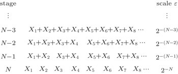
Let us now explain how to obtain the weights w_i from a positive time series. The basic idea in analyzing a generic time series {X_i} is to view {X_i, i = 1,…, 2^N} as the weight series of a certain multiplicative process at stage N. Under this scenario, the total weight is set equal to 1 unit, and the scale associated with stage N is ε = 2^–N. This is the smallest time scale resolvable by the measured data.

Given the weight sequence at stage N, the weights at stage are obtained by simply adding the consecutive weights at stage N over nonoverlapping blocks of size 2, i.e., for i = 1,…,2^{N – 1}, where the superscript 2¹ for is used to indicate that the block size used for the summation at stage N – 1 is 2¹. This follows directly from the construction of a multiplicative multifractal process schematized in Fig. 5. Associated with this stage is the scale ε = 2^–(N–1). This procedure is carried out recursively. That is, given the weights at stage we obtain the weights at stage by adding consecutive weights at stage j + 1 over nonoverlapping blocks of size 2, i.e.,

Fig. 5.

	Figure Option ViewDownloadNew Window
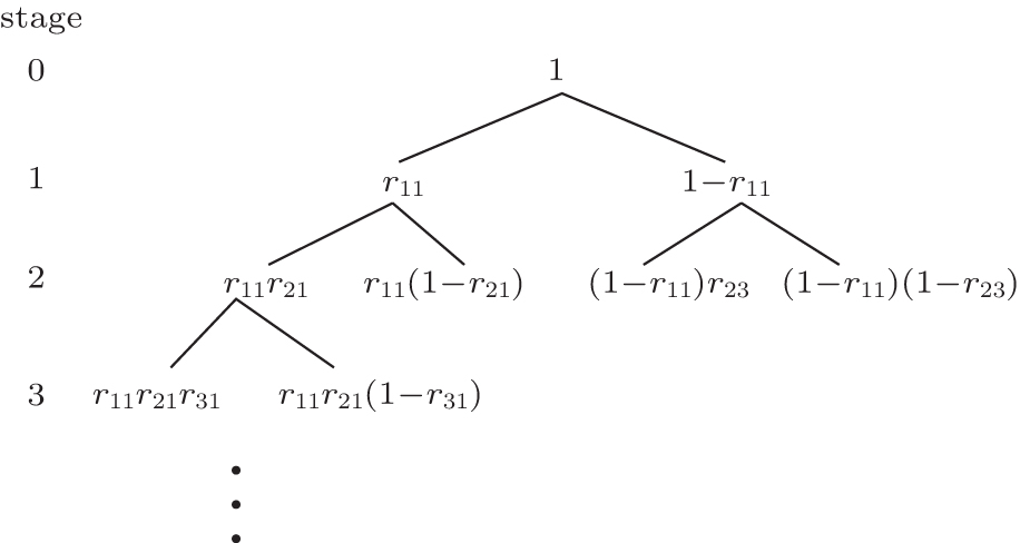	Fig. 5. Schematic of the construction rule.

Fig. 6.

	Figure Option ViewDownloadNew Window
	Fig. 6. Schematic for obtaining weights from a time series.

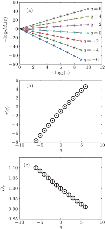
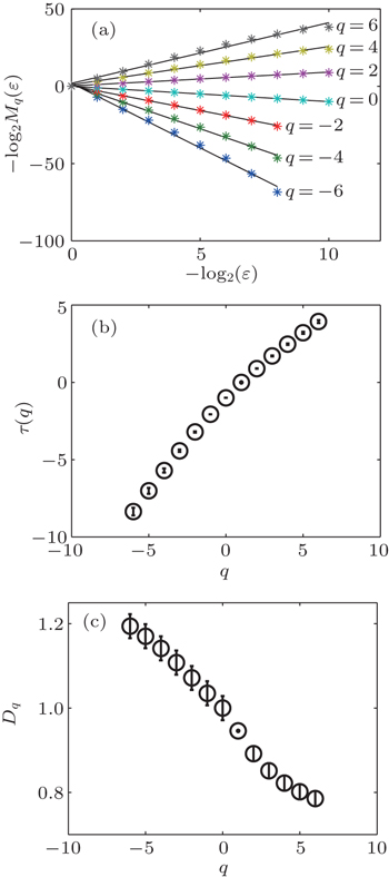
Following the above procedure, we have analyzed the multifractal properties of x₁ and x₂. The results are shown in Figs. 7(a) and 8(a), respectively. We observe that the scaling behaviors are very good. The τ(q) and D(q) spectra are shown in Figs. 7(b), 7(c) and 8(b), 8(c), respectively. Clearly, both the time series of the color and the clarity degree have multifractal behavior.

Fig. 7.

	Figure Option ViewDownloadNew Window
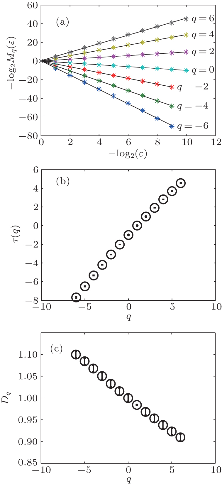	Fig. 7. Multifractal analysis of the time series data of color value. Fitted lines for (a) Eq. (5), (b) τ(q), and (c) Dq.

Fig. 8.

	Figure Option ViewDownloadNew Window
	Fig. 8. Multifractal analysis of the time series data of clarity degree. Fitted lines for (a) Eq. (5), (b) τ(q), and (c) Dq

The relevance of the cascade multifractal model to the variations in the color and the clarity degree can be made stronger by actually simulating these variables using the cascade model schematized in Fig. 5. For this purpose, we have used a bell-shaped PDF for the multiplier

The range in the unit interval means that it is a truncated Guassian distribution, therefore, given σ, c is determined by the condition As the time series generated by the cascade model is random, to facilitate a comparison with the measured data, we have re-ordered the generated time series according to the order of the magnitude of each measurement. The results for the simulated color and the clarity degree are shown in Figs. 2(b) and 3(b). We observe that the simulated time series look very similar to the original ones. Indeed, they have very similar distributions, as shown in Fig. 4.

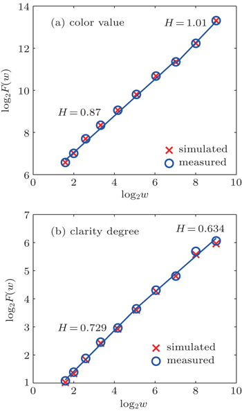
The similarity between the observed and the simulated color and clarity degree data can be further analyzed by examining the long-range correlation property of the data, quantified by the Hurst parameter 0 < H < 1. It is well-known that depending on whether H < 1/2, = 1/2, or > 1/2, a time series is said to have anti-persistent correlation, short-range correlation or is memoryless, or long-range correlations. In Ref. [1], we have analyzed the color and the clarity degree data, as well as other variables pertaining to the clarification process using detrended fluctuation analysis (DFA)^[34] and adaptive fractal analysis (AFA).^[35–38] Here, we only present the results in Fig. 9, leaving the details of DFA and AFA to the reference. Clearly, we observe that the measured and the simulated data have an almost identical long-range correlation property, for time scales up to at least a few days.

Fig. 9.

	Figure Option ViewDownloadNew Window
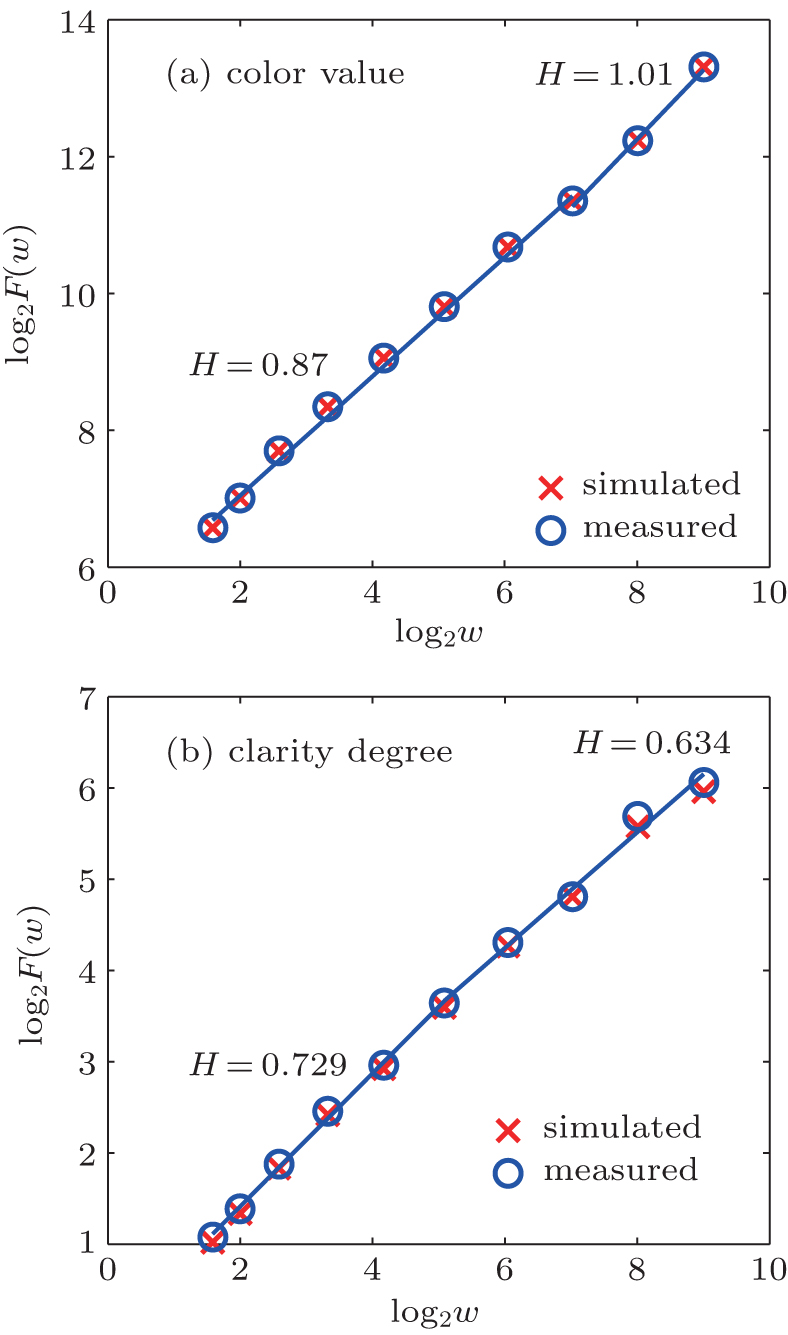	Fig. 9. Long-range correlation analysis of the measured and simulated data. (a) Color value and (b) clarity degree.

In summary, we have shown that the measured color value and clarity degree data possess multifractal properties, and can be well-modeled by the cascade process, in the sense that the distributions and the correlations of the simulated data are almost identical to those of the real data. Interestingly, these features are largely preserved when different functionals are used for the multiplier distribution, including a double-exponential

Cane sugar production is an important industrial process. One of the most important steps in cane sugar production is the clarification process, which produces high quality, concentrated sugar syrup crystal for further processing. To gain fundamental understanding of the physical and chemical processes associated with the clarification process, and help design better approaches to improve the clarification of the mixed juice, in this paper, we have examined whether the degradation in the color and the clarity degree may have system-wide causes. We have found that the answer is positive. This has further motivated us to employ the cascade multiplicative multifractal model to analyze the variations in the color and the clarity degree. We have shown that those variations can be characterized by multifractal processes. Moreover, they can be conveniently modeled by the cascade model, with the simulated and the observed data having very similar distributions as well as long-range correlation properties.

Broadly speaking, the degradation in the color and the clarity degree may be thought to be caused by the “impurities” in the sugarcane. The cascade model adopted here is essentially a conservative model. This suggests that the “impurities” in the sugarcane may be associated with the “remnants” of the “dirts” of all kinds that remain during the initial cleaning of the sugarcane. Referring to the construction rule of the cascade model shown in Fig. 5, this means that the impurities throughout the entire cane sugar production process can be thought of as coming from the partition of the total impurity (of 1 unit), with the partition rule governed by the multiplier distribution. We surmise that the total impurity is largely introduced by the in-effectiveness in cleaning up the sugarcane in the initial step. If this is so, then to improve clarification, it will be beneficial to use a more powerful cleaning system and filters to better clean up the sugarcane and raw juice. If too much of the impurities are generated by the middle steps during cane sugar production, then the whole cane sugar production process has to be considered fundamentally flawed and in-effective.