1. IntroductionA classic problem in electric circuit theory that has been extensively studied for more than 170 years is the computation of the resistance between two arbitrary nodes in a resistor network.[1] Resistor networks have been widely studied and simulated as models for many problems in science and engineering.[2–30] In particular, some practical problems have been solved by making use of the network models.[24–30] In the process of study on the arbitrary resistor networks, the theory and methods of studying resistor network are constantly developed. So far three main methods have been developed.[5,8,18–20]
Before 2004 research focused mainly on infinite lattices and the use of Green’s function technique.[5–7] Little attention has been paid to finite networks, even though the latter are those occurring in real life. It was not until 2004 that Wu[8] revisited the resistance problem of the resistor network and established a theorem based on which the equivalent resistance between any two nodes in a resistor network can be computed by using the Laplacian approach. For the m × n network the results are in the form of a double summation. Additional work is required to reduce this into a single summation. It is necessary to emphasize that Green’s function technique cannot solve the problem of finite resistor network, and Laplacian approach is confined to regular lattices with regular boundary (such as free, periodic or zero resistor boundary, etc.), which cannot solve the problem of resistor network with arbitrary boundary.
At present, a new recursion-transform (RT) method has been established[18–20] which makes up for the disadvantages of the above two methods; the RT method can compute the equivalent resistance of an m × n resistor network with arbitrary boundary and express the resistance directly in a single summation.
By the RT method many resistor networks of various topologies are resolved, such as a cobweb model,[11–14] a globe network,[15] a fan network,[16] a cobweb network with 2r boundary.[17] This method was further improved in 2015,[18–20] which, now, can be applied to a resistor network with arbitrary boundaries.
As is well known, the regular boundary is an idealized condition but the arbitrary boundary is realistic and in practical cases. The search for the exact solutions of resistance is important but difficult when the boundary is an arbitrary resistor, since the boundary is like a wall or trap which affects the behavior of finite network. This paper focuses on studying the problem of the two-point resistance in a rectangular m × n resistor network with an arbitrary boundary, which has never been solved before, and in this paper a general formula is obtained and eight interesting results are deduced. At the same time the resistance results are applied to the complex impedance network. As is well known, the research of complex impedance network is more difficult than that of the resistor network, because the equivalent impedance has many different properties from equivalent resistance. From previous studies of the equivalent impedance we find that the results of the equivalent complex impedance are always curious and nonlinear.[9,11,21–23] Thus complex impedance is an important problem worthy of study.
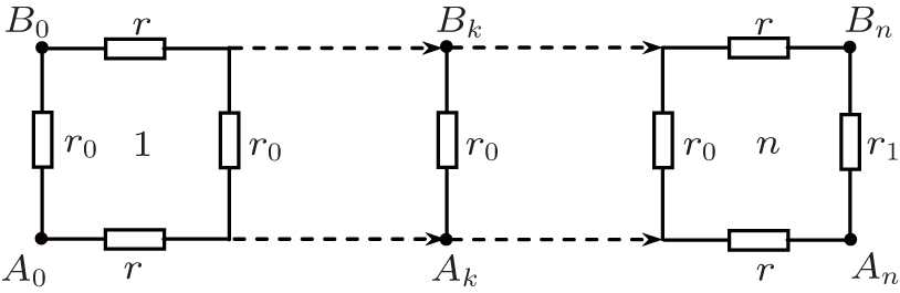
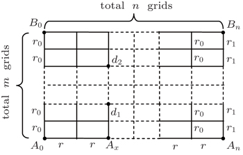
Figure 1 shows a rectangular m × n resistor network with an arbitrary boundary, where m and n are the grid numbers respectively in the vertical and horizontal directions, and r0 and r are the resistor elements in the respective vertical and horizontal directions, and r1 is the resistor at the right boundary. This paper focuses on finding the equivalent resistance Rm×n (d1,d2) in the resistor network, in which d1 (x,y1) and d2 (x,y2) are two arbitrary nodes on a common vertical axis of the m × n resistor network. We also study the characteristics of the equivalent impedance of the RLC network by the equivalent resistance formula.
The rest of this paper is organized as follows. In Section 2, we present an exact formula of resistance between two arbitrary nodes on a common axis for both finite and infinite rectangular network. In Section 3, we prove the exact formula of the equivalent resistance by the RT method. In Section 4, several specific resistance formulae are derived by the general formula. In Section 5, the equivalent impedance of the RLC network is studied by using the resistance formula. Section 6 gives a summary and discussion for the method and results.
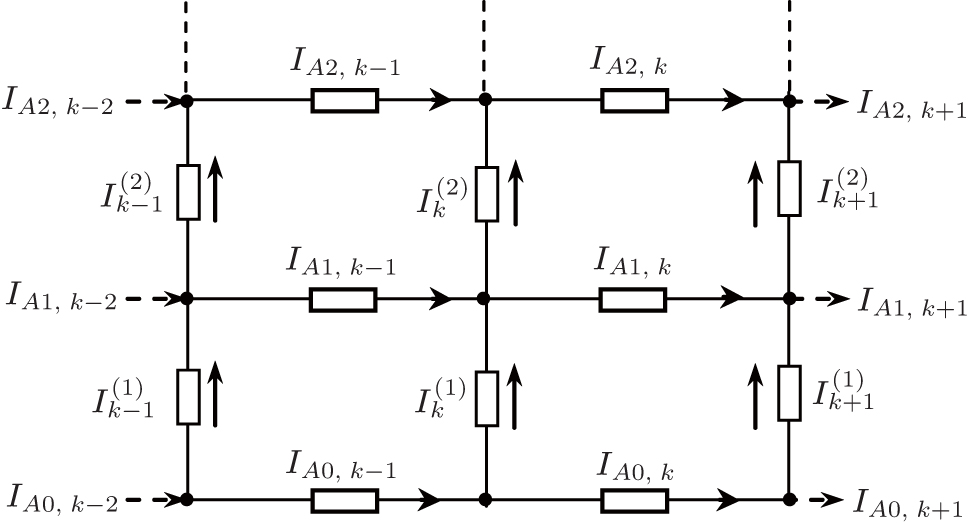
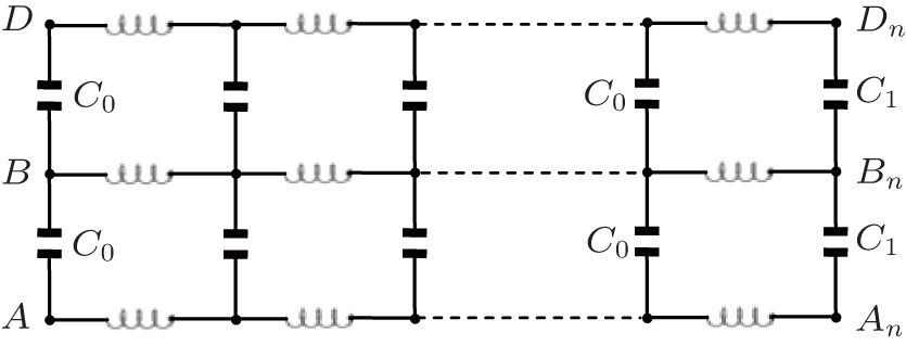
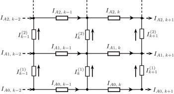
3. Derivation of the main formula3.1. Modeling the matrix equationWe denote nodes of the network by coordinate (x, y) as shown in Fig. 1. We assume that the current J is constant and goes from the input d1(x,y1) to the output d2(x,y2). Denoting the currents in all segments of the network as shown in Fig. 2, the branch currents flowing through all horizontal resistors r’s in the (m+1)th row are, respectively, IA0,k, IA1,k, IA2,k, …,IAm,k (1 ≤ k ≤ n); the currents flowing through all vertical resistors r0’s in the (n + 1)th column are, respectively:  (0 ≤ k ≤ n).
Using Kirchhoff’s law (KCL and KVL) to analyze the resistor network, the node current equations and the mesh voltage equations can be achieved from Fig. 2. We therefore obtain the relations as follows (readers may refer to Refs. [11] and [14]–[20]):
Equation (4) can be written in a matrix form after considering the following input and output current:

where
Ik and
Hx are respectively
m × 1 column matrix, and read


where [ ]
T denotes matrix transpose, and (
Hx)
i is the elements of
Hx with the injection of current
J at
d1(
x,y1) and the exit of current
J at
d2(
x,y2), and
where
r/
r0 =
h. Equations (
5)–(
8) constitute the main matrix equation model of the
m ×
n resistor network.
3.2. General solution of the matrix equationAs equation (5) is a complex matrix equation, we cannot direct acquire its solution. How to solve the matrix Eq. (5) is the key to the problem. We rebuild a new difference equation and solve Eq. (5) indirectly. To realize the idea, first, we multiply Eq. (5) from the left side by an m × m undetermined square matrix Pm, and obtain

Constructing the transformation of diagonal matrix by the following two identities:

where diagonal matrix
Tm = diag(
t1,
t2, …,
tm). Solving Eq. (
10), we obtain
[11,14–20]

where
θi =
iπ/(
m + 1), and
with the inverse matrix

For convenience, by Eqs. (9) and (10) we appoint

Thus we obtain the following equation after making use of Eqs. (9), (10), and (14):

where
Supposing that λi and  are the roots of the characteristic equation for Xk, from Eq. (15) we obtain Eq. (3).
Next, we consider the solution of Eq. (15) when injecting current J at d1(x,y1) and exiting current J at d2(x,y2). We obtain the piecewise solutions of Eq. (15) as


where

is defined in Eq. (
2).
3.3. Boundary conditions of currentWe consider the boundary conditions of the left and right edges in the resistor network. Using Kirchhoff’s law (KCL and KVL) to analyze the resistor network, and adopting the method similar to that of establishing Eq. (1), we obtain three matrix equations to model the boundary conditions, which are

where
h1 =
r1/
r0, and
Em is the
m ×
m identity matrix, matrix
Am is given by Eq. (
8).
Conducting the same matrix transformation as that in Eq. (9), applying Pm to the left-hand side of each of Eqs. (20) and (21), we have


Combining Eqs. (17)–(19), (22), and (23), we obtain after some algebra and reduction the solution needed in our resistance calculation (see Appendix A)
where
ζi is defined in Eq. (
16), and
ti is given by Eq. (
11). Formula (
24) is a key solution for computing current

because

is a function of

(see Eq. (
14)).
3.4. Final step of derivationTo calculate the equivalent resistance Rm × n (d1, d2), we first consider current  . Taking the inverse transformation of Eq. (14) with k = x, we have
  , i.e.,
From Eq. (25), we obtain

Substituting Eq. (24) into Eq. (26), we obtain
where
is used.
Since voltage  , by Ohm’s law we have
Substituting Eq. (27) into Eq. (28), we obtain formula (1).
4. Several specific resistance formulaeFormula (1) is a general resistance expression. As applications, from formula (1) we can deduce several interesting new results. In this section, we will give several specific resistance formulae in both finite and infinite networks.
Case 1 When h1 = 1, the resistor network of Fig. 1 degrades into a regular m × n rectangular resistor network, from Eq. (1) we have
Case 2 When d1 and d2 are both at the left edge, from Eq. (1) we have the resistance on the left edge
Since  , we therefore rewrite formula (30) as
In particular, when h1 = 1, from formula (31) we have
Case 3 When n → ∞, but m and x are finite, figure 1 turns into a semi-infinite resistor network: the grid number along the right direction is infinite but along the vertical direction is finite. From formula (1) we have
Derivation process is as follows.
When n → ∞ with m being finite, by using Eqs. (2) and (3), the factor on the right-hand side of formula (1) can be reduced into
where
a = (
λi +
h1 − 1) and

. By using Eq. (
3) we know

, thus
Substituting Eq. (35) into formula (1) with n → ∞, we obtain formula (33) after using  .
.
Case 4 When m → ∞, but n, y1, and y2 are finite, which means that Fig. 1 turns into a semi-infinite resistor network: the grid number along the upward direction is infinite but along the horizontal direction is finite, we have the equivalent resistance as follows:
where
Ck = cos (
yk + 1/2)
θ, and
with

. Derivation process is as follows.
When m, n → ∞, for proving Eq. (36), we need an integral theory as follows.
If θk = ukπ/(m + 1), we have Δθk = θk+1 − θk = uπ/(m + 1). In the case of m → ∞, we have

which is an identity valid for any function
g(
θk). Equation (
37) is prepared to prove Eqs. (
36), (
38), and (
40)–(
42) in the following.
When m → ∞ but n,x and y1,y2 are finite, as θk = k/(m + 1)π in Eq. (1), and λi is a function of θi, thus, making use of Eq. (37) we convert the summation of formula (1) into an integral (36), so formula (36) is proved.
Case 5 When m → ∞, y1,y2 → ∞, but n and y1 − y2 are finite, figure 1 turns into a semi-infinite resistor network: the grid number along the vertical direction is infinite but along the horizontal direction is finite, we have the equivalent resistance
Derivation process is as follows. According to the identity transform of a trigonometric function, we have

When m → ∞ and y1, y2 → ∞, we may transform

where
p,
q ≪
m are integers, and (
p −
q) = (
y1 −
y2) are finite, we therefore have
From Eq. (2) we have Δθ2k−1 = θ2k+1 − θ2k−1 = 2π/(m + 1). Thus applying Eqs. (37) and (39) to formula (1), we obtain integral (38).
Case 6 When m,n → ∞ with x being finite, figure 1 turns into an infinite resistor network, but the network along the left direction is finite, we have
where

. Derivation process is as follows.
When m,n → ∞ and y1,y2 → ∞, we have Eqs. (35) and (38). First, we have Eq. (35), then apply Eq. (35) to Eq. (38) and we obtain integral (40).
When x → ∞, as  , we have
  , thus from Eq. (40) we immediately obtain the following formula.
Case 7 When m,n → ∞, and x → ∞, which means that figure 1 turns into an infinite resistor network, the grid number along both the vertical and horizontal direction are infinite, we have the equivalent resistance
When x = 0, as  , thus from formula (40) we immediately obtain the following formula.
Case 8 When m,n → ∞ with x = 0 finite (means d1 and d2 are both on the left edge), we have the equivalent resistance
Note that formula (1) and cases 1–8 in this paper are given for the first time. The above eight special cases illustrate that formula (1) is a multifunctional formula of equivalent resistance, which provides a clear way for practical applications, and can help readers understand in depth the connotation and the physical significance of formula (1).
In the following, we continue to give several results of a simple example to test the reliability of formula (1).
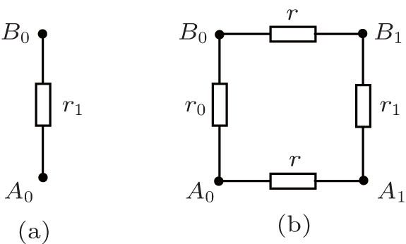
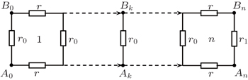
Case 9 When m = 1, figure 1 reduces into a 1 × n resistor network with an arbitrary right boundary as shown in Fig. 3. When we compute the resistance between two nodes Ak (k,0) and Bk(k,1), we have y1 = 0, y2 = 1, and i = 1. Thus from θi = iπ/(m + 1) we have θ1 = π/2, and  ,
,  , and
, and

From formula (1), we obtain the resistance as follows:
In particular, when setting k = 0, from Eq. (44) we obtain a simple result
Because  , we have

Thus, when n = 0, from Eq. (45) we have
When n = 1, from Eq. (45) we have
Obviously, formulae (46) and (47) are completely in accordance with the results of the actual circuit as shown in Fig. 4. In particular, when h1 = 1, the result obtained from formula (45) is completely in accordance with the result of Ref. [11]. These test results demonstrate the validity of the main formula (1). In fact, the results we obtained are inevitably perfect since all of the processes of algebra and reduction are strict and self-consistent.
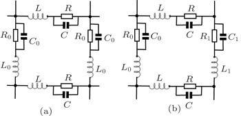
5. Equivalent impedance of the RLC network5.1. Impedance formula of the RLC networkIn Fig. 1, the grid elements are arbitrary, which can be either a resistor or an impedance. If the grid elements are complex impedances, we call the model an m × n complex impedance network, and its segment grid of impedance network is shown in Figs. 5(a) and 5(b). We assume that the alternating current (AC) frequency is ω, then there must be the following mapping relations:
where i
2 = − 1. By substituting Eq. (
48) into formula (
1) we obtain the equivalent impedance of an
m ×
n complex RLC network. Thus the general formula of the equivalent impedance between two arbitrary nodes
Ap(0,
p) and
Aq(0,
q) at the left boundary of an
m ×
n rectangular RLC network can be written as
where
θi =
iπ/(
m + 1),
Ck,i = cos (
yk + 1/2)
θi, and
fn (
λi,
h1) is defined as

with

Obviously, the characteristics of the equivalent impedances of Zm×n (Ap,Aq) will be determined by the corresponding function of fn(λi,h1). Thus we will first study the characteristics of the function of fn (λi,h1).
Since formula (49) is expressed in a complex form, it therefore is more valuable and can be more useful than the resistance formula. Although the unit complex impedance in Fig. 5 is quite complicated, formula (49) is simple. Many properties on the equivalent impedance can be derived from expression (50).
5.2. Results of the special conditionsIf 1 + h − hcos θi = − 1, we have hsin2(θi/2) = − 1, thus from Eq. (51) we obtain λi = − 1, substituting it into Eq. (52) we have
where
θi =
iπ/(
m + 1). In this case we derived that
If h1 = 1, from Eq. (55) we obtain

Namely, when equation (54) is established, some special results can be obtained by using Eq. (50).
In particular, if R = R0 = ∞ and L = L0 = 0, we have h = C0/C, thus we call Fig. 1 an m × n capacitance network. We know the equivalent capacitance to be Cn ↔ −i/(ωCn), then we can easily obtain the equivalent capacitance from formula (49).
Formula (49) is concise and significant, but it is complicated to understand the essential meaning of the RLC network because the special condition of the parameters RLC needs to be considered in order to find its application value. In some special applications, the readable results can be obtained if the impedance parameters have some specific values. The usefulness of formula (49) is best illustrated by application examples. One application is now given below.
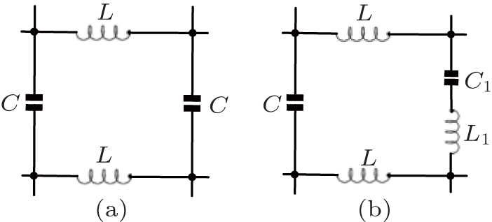
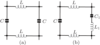
5.3. Equivalent impedance of the LC networkConsider an m × n impedance LC network, from formula (49), then we will be able to obtain the equivalent impedance of a rectangular m × n LC network. Assuming that the impedance elements of the horizontal and vertical directions in lattice are r = iω L, r0 = 1/iωC, and r1 = iωL1 + 1/iωC1 as shown in Figs. 6(a) and 6(b) respectively, the equivalent impedance between two arbitrary nodes Ap (0,p) and Aq(0,q) at the left boundary of an m × n LC network is given by
where
θi =
iπ/(
m + 1),
fn(
λi,
h1) is defined in Eq. (
50), and


In Eq. (59) the λi is worthy of discussion as h is a negative number. For example, 1 + h − hcosθi = − 1, there is λi = − 1, by using Eq. (59), we have
in this case we obtain

In the case of  , we have
Thus, by using Eqs. (58) and (62) we obtain

with

As a result, we have

In the case of  , substituting Eq. (64) into Eq. (57), we have
In the case of

substituting Eq. (
64) into Eq. (
57), we have
The above analysis illustrates that equivalent impedance formula is more complicated, which is quite unlike the resistance network, and needs to consider a variety of conditions and the equation root of a complex situation as well.
5.4. Circuit resonance conditionsAn important feature of the complex impedance network is that its circuit can resonate under certain conditions, which is completely different from the resistor network. For example, when sin(n + 1)ϕi + (h1 − 1) sin nϕi = 0, we have

where
ϕi = arccos [1 − 2
ω2LCsin
2(
θi/2)] is defined in Eq. (
63). Substituting Eq. (
59) into Eq. (
67), we have

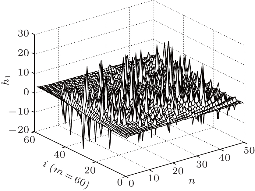
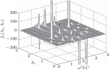
When equation (68) holds, we find that Eqs. (65) and (66) are in resonance. In the case of ω2LC = 1 we draw the 3D graphics to clarify the specific relationship for Eq. (68) as shown in Fig. 7, which illustrates the relationship among h1 and i (1 ≤ i ≤ m = 60) and n (n ≤ 50).
Figure 7 shows that there are many h1 values that can satisfy Eq. (68), that is to say, a case which can occur at a specific frequency ω in an AC circuit, then the effective impedance (57) between two nodes Ap (0,p) and Aq (0,q) diverges and the network is in resonance. Since L1 and C1 are the right boundary elements which can be controlled artificially, we therefore can adjust L1 and C1 to lead to the result in resonance circuit. In other words the external boundary conditions affect the circuit resonance conditions, which is an interesting conclusion. In these cases, boundary condition of h1 with the frequency ω of an external AC source can cause the resonance in the LC circuit, which can be calculated by using Eq. (68). Thus we can control the circuit resonance by controlling the L1 and C1. This curious result suggests the possibility of practical applications to resonant circuits.
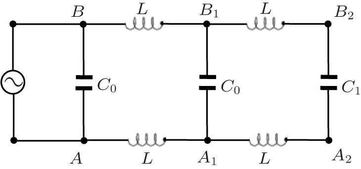
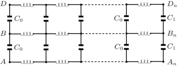
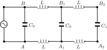
5.5. Equivalent impedance of the 2×n LC networkStudy of the complex impedance networks is usually complicated. In order to reveal more characteristics of the impedance network, we restrict ourselves to the simple model as shown in Fig. 8. Assuming that the AC frequency is ω, then the general equivalent impedance of 2 × n LC network with an arbitrary capacitance can be deduced from Eq. (57) as

where
fn (
λ1,
h1) is defined as
with

and
h = −
ω2LC,
h1 =
C/
C1.
Equation (70) is the general formula of the 2 × n impedance LC network which can be applied to a variety of cases such as the following examples. We just show that by formula (70) itself its meaning and characteristics cannot be sufficiently understood. Hence, we must consider the amplitude–frequency characteristics of fn(λ1,h1) and investigate the resonance characteristics.
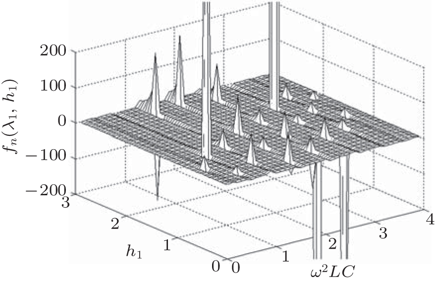
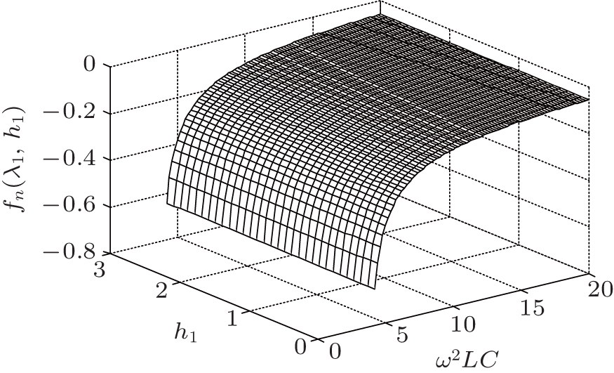
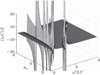
5.6. Amplitude–frequency characteristics of fn(λ1,h1)There are four parameters in the function of fn(λ1,h1), we set n = 10, the 3D graphics of the complex impedance function of fn(λ1,h1) changes with ω and h1 as shown in Figs. 9 and 10. Figure 9 shows that fn(λ1,h1) has occasional oscillation and resonance. Figure 10 shows that fn(λ1,h1) is gradually increasing with the increase of ω2LC when ω2LC > 4.
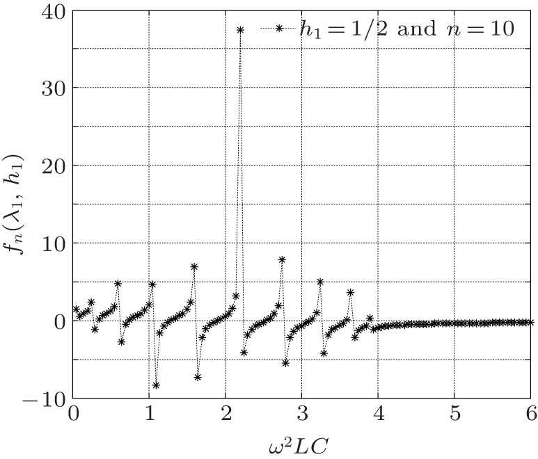
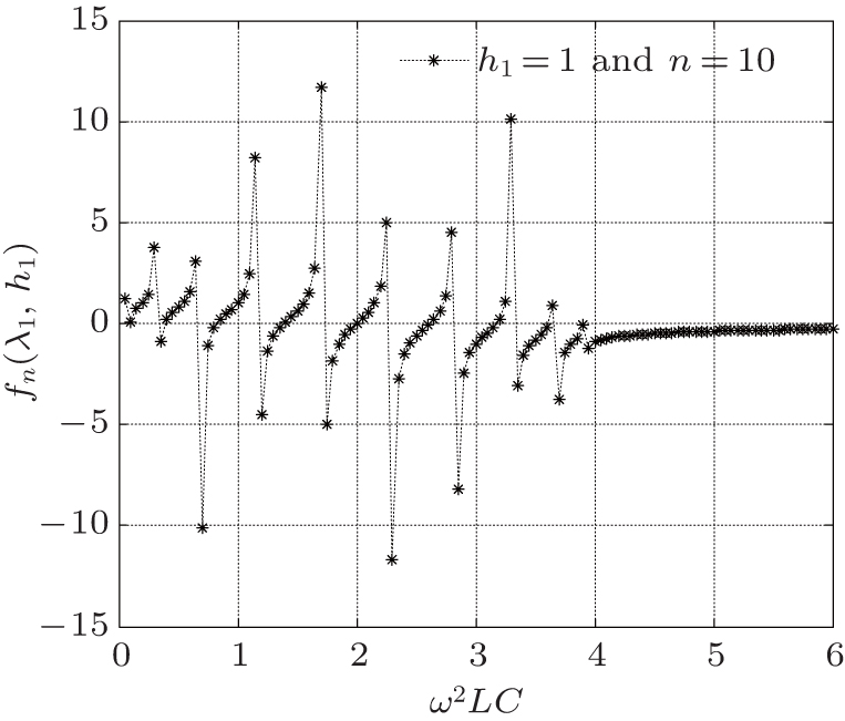
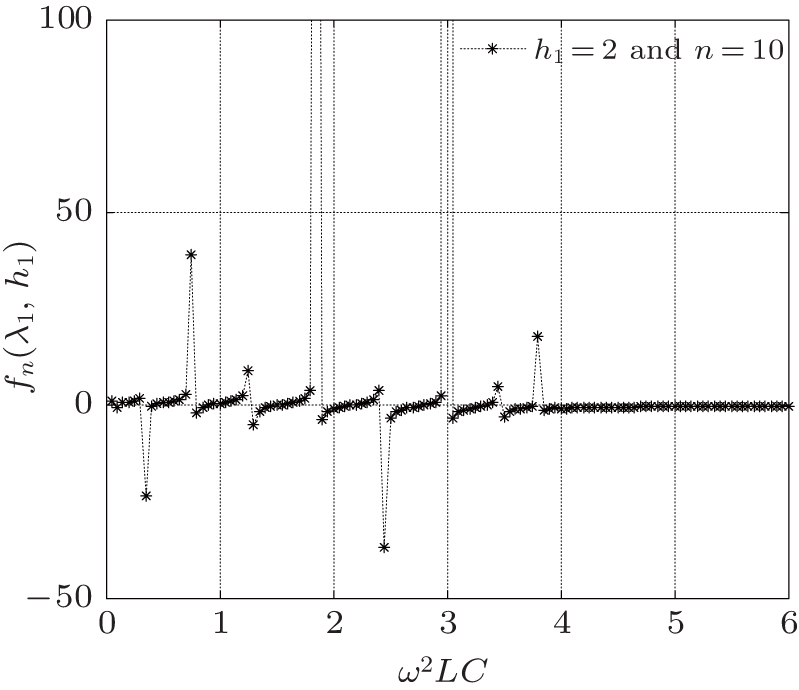
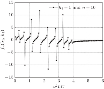
These 3D graphs of Figs. 9 and 10 show the overall situation, but for clearly seeing characteristics we draw the 2D graphs. For example, setting n = 10 and h1 = 0.5,1,2, the complex impedance function of fn(λ1,h1) changes oscillatorily with ω as shown in Figs. 11–13.
These 2D graphs of Figs. 11 and 12 are interesting because their changes are aperiodic but look like being periodic. Figure 13 shows that fn(λ1,h1) has occasional resonance.
5.7. Impedance formulae in different conditionsCase 1 Under the condition of  , we know
  , therefore, when n → ∞, taking the limit of Eq. (2) yields,
Substituting Eq. (71) into Eq. (69), we obtain

Equation (72) gives the equivalent impedance of a semi-infinite 2 × n LC network, and the grid number along the right direction is infinite but along the left direction it is finite.
Case 2 Under the condition of  , there is λ1 = − 1, we have Eq. (61). Substituting it into Eq. (69), we have

Case 3 Under the condition of  , from Eq. (63) we have
As a result, we have Eq. (64), so substituting Eq. (64) into Eq. (69), we obtain
Formula (75) clearly shows that the complex impedance has nonlinear characteristics, the chaotic characteristics, and resonance features.
Obviously, when we investigate the characteristic of Eq. (69), we will find that the characteristic of Z2×n (A,D) changes unsteadily with n and h1. The above equations are the personalized formulae under the different conditions, which show the analysis formulae of the equivalent complex impedance in the LC network are complicated.
In the following we continue to take a simple example to illustrate the resonance of a simple LC network.
Case 4 We consider a 1 × n LC network with an arbitrary boundary. Assuming that AC frequency is ω, the equivalent impedance of 1 × n LC network with an arbitrary capacitance can be deduced from Eq. (57) as
where

,

, with
h = −
ω2LC and
h1 =
C/
C1.
In particular, when we consider a 1 × 2 LC network as shown in Fig. 14, from formula (76) we have
Simplifying Eq. (77) yields
Since  , substituting it to Eq. (78) gives
Consider the condition of resonance circuit, assume that the denominator of Eq. (79) is zero, then we will have

Equation (80) indicates that there are many C1’s that can satisfy Eq. (80). In this condition the effective impedance between two nodes A and B diverges and the network is at resonance. Since C1 is the element on the right edge, which can be controlled artificially, we therefore can adjust C1 to lead to the result in resonance circuit.
In order to intuitively show that C1 controls the circuit resonance, we describe two figures to illustrate the resonance features of Z1×2(A,B) in Figs. 15 and 16. The 3D graph of the complex impedance of Z1×2(A,B) changes with ω and h1. Figure 15 illustrates the resonance nodes, and figure 16 displays the enlarged part of the graph in Fig. 15.
6. Summary and discussionIn this paper a general resistance formula (1) is derived by the RT method for a rectangular m × n network with an arbitrary boundary (see Fig. 1), and formula (1) is found for the first time. As applications, eight interesting specific results of the resistor network are derived. Further, the current distribution is given explicitly as a byproduct of the method. Our framework is effectively applied to the complex impedance networks. The above is our main contribution. In the process of research to obtain the solution of Eq. (5) is the key and also a difficult job. We solve this problem by the matrix transformation method.
As is well known, the study of complex impedance network is more complex than resistor network, because the equivalent complex impedance is related to the frequency of the input circuit. We study the equivalent impedance of a rectangular m × n impedance network between Ap and Aq with an arbitrary boundary, which has never been resolved before. The advantage of the arbitrary boundary is that it can be artificially controlled to design a control circuit. The analyses of chaos characteristic and resonance properties are mainly based on the frequency and the element r1 on the right edge (see Eq. (68)). In the RLC network, our formulation leads to the occurrence of resonances under the boundary condition where it holds a series of special values with an external AC source (see Fig. 7). This somewhat curious result suggests the possibility of practical applications of our formulae to resonant circuits.
The characteristic of the equivalent impedances is determined by the function fn(λi,h1) which is defined in formula (50). When R = R0 = ∞ and L = L0 = 0, we can obtain the equivalent capacitance of an m × n capacitance network and its equivalent capacity is Cn ↔ −i/(ωCn), which can be deduced from formula (49).
As a next step, we consider an m × n impedance LC network and its equivalent impedance is given by formula (57). An important property of complex impedance network is the circuit resonance and this phenomenon is illustrated in the 3D graph of Fig. 9.
Finally, we detail the 2 × n LC network and illustrate the features of the amplitude–frequency characteristics of the function fn(λ1,h1) as a function of ω and h1 in a 3D graph as shown in Figs. 9 and 10. Specifically, we find that the equivalent impedance of Z2×n(A,D) increases gradually with the increase of ω when the value of ω2LC is big enough such as ω2LC > 4, which has no oscillation as shown in Fig. 10, while in Figs. 11–13 three 2D graphics are obtained for the specified values of n and h1. The complex impedance function fn(λ1,h1) varying with ω is clear from Figs. 11–13. In particular, we give a 1 × 2 LC network to illustrate that the circuit resonance can be controlled by controlling boundary capacitance C1.
The above study shows that the equivalent impedance has many different properties from equivalent resistance, and these properties of oscillation and resonances suggest the possibility of practical applications of our formulae to real life.


 ]
]