Quantum information entropy for one-dimensional system undergoing quantum phase transition
Song Xu-Dong1, Dong Shi-Hai2, Zhang Yu3, †,
Software Institute, Dalian Jiaotong University, Dalian 116028, China
CIDETEC, Instituto Politécnico Nacional, Unidad Profesional ALM, Mexico D. F. 07700, Mexico
Department of Physics, Liaoning Normal University, Dalian 116029, China


† Corresponding author. E-mail: dlzhangyu physics@163.com

Project supported by the National Natural Science Foundation of China (Grant No. 11375005) and partially by 20150964-SIP-IPN, Mexico.

Abstract
Abstract

Calculations of the quantum information entropy have been extended to a non-analytically solvable situation. Specifically, we have investigated the information entropy for a one-dimensional system with a schematic “Landau” potential in a numerical way. Particularly, it is found that the phase transitional behavior of the system can be well expressed by the evolution of quantum information entropy. The calculated results also indicate that the position entropy Sx and the momentum entropy Sp at the critical point of phase transition may vary with the mass parameter M but their sum remains as a constant independent of M for a given excited state. In addition, the entropy uncertainty relation is proven to be robust during the whole process of the phase transition.

1. Introduction

Recently, there has been a growing interest in dealing with information theoretical measures for quantum-mechanical systems. As an alternative to the Heisenberg uncertainty relation, entropic uncertainty has been particularly examined.[13] Among the measures of information entropy, Shannon entropy[46] plays a very important role in the measure of uncertainty, which has been tested for various forms of potentials. The entropic uncertainty relation, which is related to the position and momentum spaces, was given by[79]

where D represents the spatial dimension. In the one-dimensional system, the position-space (Sx) and momentum-space (Sp) information entropies are defined, respectively, by

where ψ(x) is a normalized eigenfunction in spatial coordinates and ϕ(p) is its normalized Fourier transform.

Apart from their intrinsic interest, the entropic uncertainty relations have been used widely in atomic and molecular physics.[1014] For example, the Shannon information entropies for a few molecular potentials have been analytically obtained, i.e., the harmonic oscillator,[15] the Pöschl–Teller (PT),[16,17] the Morse,[16,18] the Coulomb,[19] the potential isospectral to the PT potential,[20] the classical orthogonal polynomials[2123] and other studies.[2426] In addition, investigation of the quantum information entropies was also carried for other analytically solved potentials such as the symmetrically and asymmetrically trigonometric Rosen–Morse,[27,28] the PT-like potential,[29] a squared tangent potential,[30] the position-dependent mass Schröinger equation with the null potential,[31] the hyperbolic potential,[32] the infinite circular well[33] and the Fisher entropy for the position-dependent mass Schrödinger equation,[34,35] due to their applications in physics. Notably, the previous discussions related to shannon entropy were mostly focusing on analytically solvable potentials, but not all the interesting quantum systems have the corresponding analytically solvable modes. Then an efficient numerical method would be particularly important. In this work, we will extend the calculations of shannon entropy to the one-dimensional system with a schematic “Landau” potential,[36,37] which may be formally derived in the mean-field level from the vibron model for molecular structures[38,39] and can be only solved in a numerical way. Particularly, there exists a quantum phase transitional behavior in the system as varying the control parameter in this type of potential.[36,37]

2. Schematic “Landau” potential and its numerical solution

One way of addressing quantum phase transitions[40] is to use the potential energy approach. A schematic “Landau” potential is often considered to indicate quantum phase transition,[36,37] which is written as

with M being the mass parameter and β ∈ [0, 1] being the control parameter. One can prove that the minimum of V(x) with β ≤ 0.5 may locate at x = 0, while V(x) with β > 0.5 may have two degenerated minimums at x ≠ 0, which indicates that quantum phase transition may occur at the critical point β = 0.5. More specifically, it can be derived that the minimum of V(β), Vmin, and ∂ Vmin/x at the critical point β = 0.5 are continuous, but 2 Vmin/∂x2 is discontinuous, which confirms that there indeed exists a second-order quantum phase transition occurring at the critical point β = 0.5. As we know, quantum phase transition may be reflected not only by the potential surface evolution of the system but also by the low-lying dynamics properties. It is thus expected that quantum phase transition is also indicated by the information entropies. To calculate the information entropy, one has to solve the eigenfunctions ψ(x) from the differential equation

where the Hamiltonian is presently written as

It is clear that the differential equation (6) can be analytically solved in the β = 0 case, in which the potential form regains the harmonic oscillator one. The eigenfunction in the β = 0 case can be analytically written as

where Hm(z) is the Hermite polynomial and the normalized factor is given as

The corresponding eigenvalues are given as

Although the differential Eq. (6) in the β > 0 cases cannot be analytically solved, the numerical solutions can be achieved in a systematic scheme as shown below. One can formally expand the eigenfunctions of the n-th excited state ψn(x) in terms of the eigenfunctions of the harmonic oscillator given in Eq. (7) as

where are the expansion coefficients. Therefore, one has to get the coefficients at first in order to obtain the eigenfunctions ψn(x). For β = 0, the coefficient is just given as . For β > 0, one can diagonalize[41] the Hamiltonian (5) under the harmonic oscillator basis to get coefficients . The matrix element of the Hamiltonian under the harmonic oscillator basis is defined as

with i, j = 0, 1, 2,…, t. The number t should, in principle, be taken as infinite since the dimension of the Hilbert space for the infinite well V(x) given in Eq. (4) is infinite. However, one can diagonalize the Hamiltonian with β ∈ (0, 1] within a finite subspace with sufficient large-t truncation to get the coefficients accurate enough for the low-lying states.[37] Once one obtains the coefficients involved in the eigenfunction ψn(x), one can further get the following wave functions in momentum space using the Fourier transform

where Fm(p) is the Fourier transform of the harmonic oscillator eigenfunction Wm(x). It is given as

where

Within the same numerical scheme, one can also calculate all the other quantities in the position or momentum space.

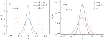
To check the validity of this method, we calculate the probability density distributions of the eigenfunctions in both the position and momentum spaces, which are defined as

The calculated results for the ground state corresponding to n = 0 are shown in Fig. 1 for three typical β values. In calculations, the mass parameter in the Hamiltonian (5) is set as M = 50 since a relatively large M value may make the phase transitional features more evident according to the analysis given in Ref. [37]. It can be found from panel (a) of Fig. 1 that the position probability density functions ρ(x) for three β values mainly distribute within the range of x ∈ [−1, 1]. Specifically, ρ(x) in the β = 0 and β = 0.5 cases may develop a peak around x = 0 except for that the peak for β = 0.5 is wider but lower than that for β = 0. In contrast, ρ(x) in the β = 1 case may develop the double-peaks structure around x = ±0.7. As further seen from Fig. 1(b), the momentum probability density function ρ(p) may converge within p ∈ [−20, 20]. Similar to ρ(x), ρ(p) in β = 0 and β = 0.5 cases also develop a single-peak but around p = 0, while ρ(p) in β = 1 case presents an evidently fluctuating behavior. In short, the different potential structure may lead to the different probability density distribution in both position and momentum spaces.

Fig. 1. Probability density distribution, ρ(x) (a) and ρ(p) (b), for the ground states with three typical β values.
3. Information entropy
3.1. Information entropy at the critical point

Once the probability density functions are obtained, the position and momentum space information entropies for the one-dimensional potential can be calculated by using Eqs. (2) and (3). Here, we will focus on discussing the situation at the critical point β = 0.5, where the system is undergoing a second-order quantum phase transition as mentioned above. The position and momentum entropy densities can be defined as

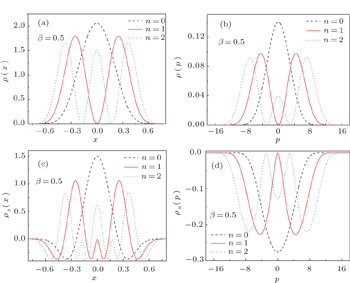
To show the properties of the information entropy densities, we plotted position and momentum entropy densities ρs(x) and ρs(p) together with the probability density functions ρ(x) and ρ(p) in Fig. 2 for the three lowest-lying states corresponding to n = 0, 1, 2. As seen from Figs. 2(a) and 2(b), ρ(x) and ρ(p) are symmetric with respect to x = 0 or p = 0 for all excited states and show a multi-peak structure: single-peak for n = 0, double-peak for n = 1 and triple-peak for n = 3. The resulting position information entropy density ρs(x) is also symmetric with respect to x = 0 for all excited states and also presents a multi-peak structure for different n number as seen in Fig. 2(c). In contrast, the momentum information entropy density ρs(p) may give an inverse multi-peak structure for different n number as shown in Fig. 2(d). Besides, the most part of the amplitude of ρs(x) is positive for a given n in contrast to ρs(p), of which the whole amplitude of ρs(p) is negative.

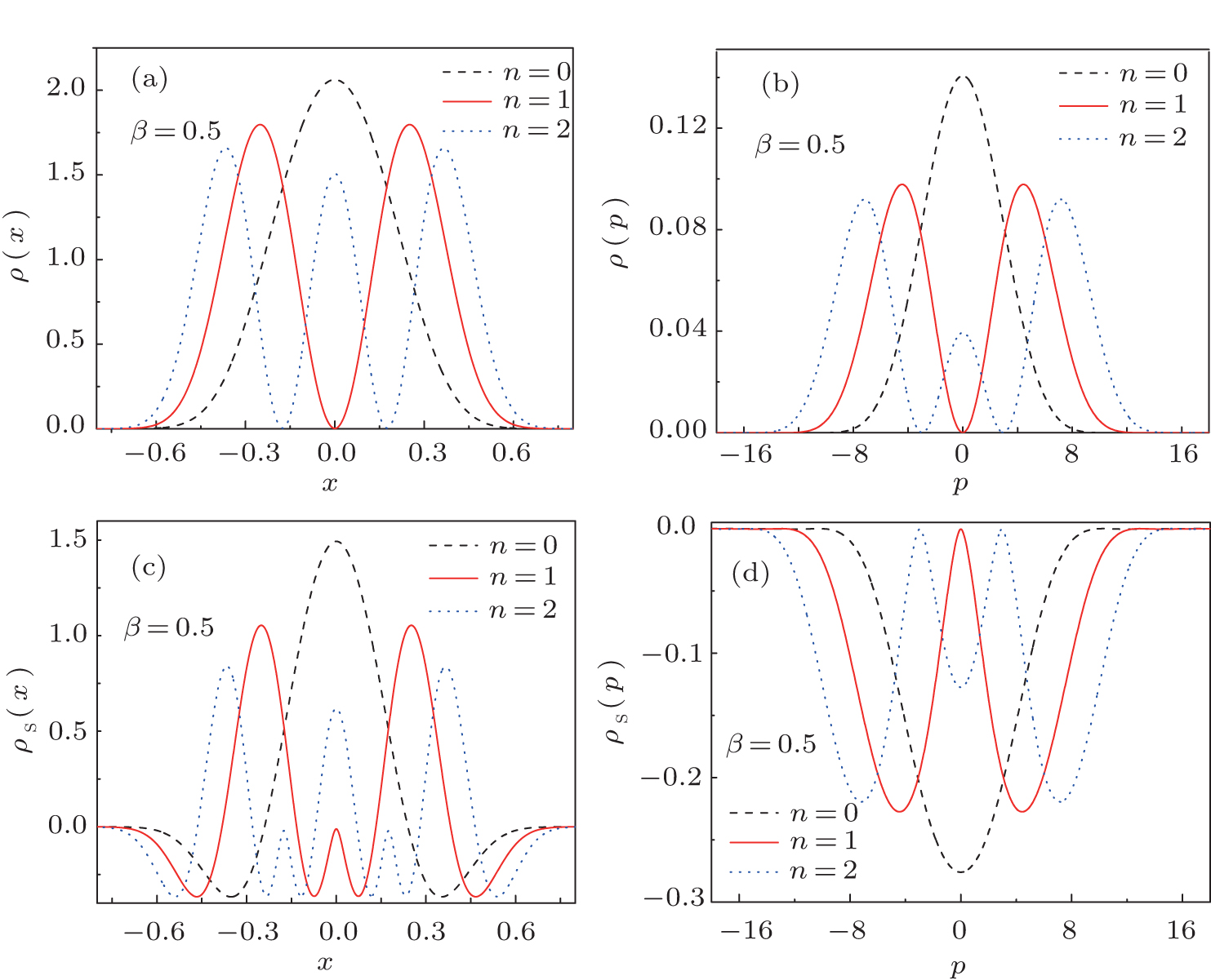
Fig. 2. Position and momentum probability densities ((a) and (b)) together with the corresponding information entropy densities ((c) and (d)) at the critical point β = 0.5 for the low-lying states with n = 0, 1, 2. In calculations, the mass parameter has been set as M = 50.

By using the information entropy densities, one can calculate the information entropies defined in Eqs. (2) and (3), which can be reexpressed as

Generally speaking, quantum fluctuations in the system around the critical point may be much larger than other situations, since the system undergoing quantum phase transition is relatively unstable. It would be interesting to find out whether the entropic uncertainty relation can be satisfied or not at the critical point. In Table l, we give the numerical results of information entropies Sx, Sp and their sum Sx + Sp with different n numbers and M values. It is clearly seen from Table l that the entropy uncertainty relation is satisfied very well in all cases. Particularly, the values of Sx might be negative in some cases, but the sum of Sx and Sp for a given n may remain as an M-independent constant, of which the value always stays above the stipulated lower bound of the value (1+lnπ).

Table 1.

Positive and momentum entropies at the critical point for the low-lying states n = 0, 1, 2 with different mass M.

.
3.2. Information entropy evolution via quantum phase transition

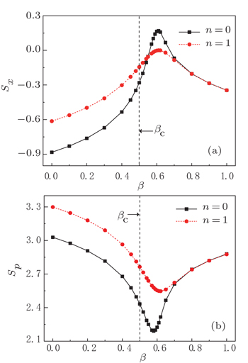
To test the transitional behavior of the information entropy within β ∈ [0, 1], the calculated results of Sx and Sp for n = 0, 1 are shown in Fig. 3 as a function of the control parameter β. As seen from Fig. 3(a), the position information entropies Sx show a non-monotonically evolution for both n = 0 and n = 1 as changing of β. Specifically, Sx may rapidly increase from negative values to positive values and then drop to negative values again with the variation of β. In contrast, the momentum information entropy Sp decreases at first and then grows up as the changing of β. More importantly, the results indicate that there is a sharp change in both Sx and Sp around the critical point βc = 0.5, which in turn indicates that the absolute value of the derivative ∂Sx/∂β or ∂Sp/∂β may reach its maximum around the critical point βc. One can thus derive that the system is undergoing a phase transition around the critical point βc. It should be noted that the turn points of Sx and Sp appearing after the critical point βc shown in Fig. 3 may rapidly approach the line denoted by βc as increasing of M, which indicate that the turn points will coincide with the line in the large-M limit.

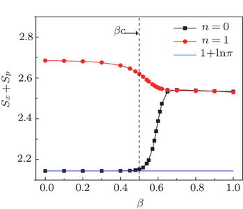
To further check the entropy uncertainty relation in the whole transitional region with β ∈ [0, 1], the results of Sx + Sp are shown in Fig. 4 as a function of the control parameter β. It can be seen from Fig. 4 that Sx + Sp may approximately remain unchanged up to the critical point β = βc = 0.5 especially for the n = 0 case, in which the value almost sustains to be equivalent to 1+lnπ before β = βc. When beyond β = βc, the results of Sx + Sp in the two cases denoted by n = 0 and n = 1 may rapidly converge to almost the same constant value as shown in Fig. 4. Anyway, the results in Fig. 4 indicate that the entropic uncertainty relation would be well satisfied during the whole process of quantum phase transition.

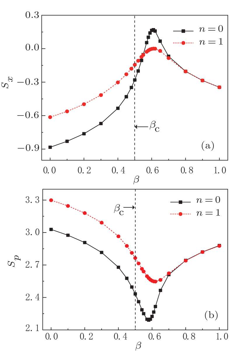
Fig. 3. The evolutions of position and momentum information entropies, Sx (a) and Sp (b) for n = 0, 1 as a function of the control parameter β, where the mass parameter is set as M = 50.
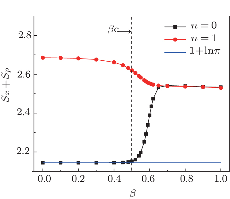
Fig. 4. The same as those in Fig. 3 but for the sum Sx + Sp.
4. Conclusion

In this paper, we have studied information entropy for a non-analytically solvable potential by adopting the diagonalization scheme. Concretely, we have investigated the properties of the position and momentum quantum information entropies of the one-dimensional system with a schematic “Landau” potential, in which the variation of the control parameter β may lead to a second-order quantum phase transition. It was found that the entropy density functions ρs(x) and ρs(p) at the critical point βc may generally give multi-peak distributions that are symmetric with respect to x = 0 or p = 0. It was also found that the results of the position and momentum information entropies Sx and Sp may change with the variations of the mass parameter M or the quantum number n but their sum Sx + Sp for a given n number remains as a constant independent of the mass parameter M. The further calculations show that there would be a rapidly non-monotonic change in both Sx and Sp around the critical point βc, which justifies that the quantum phase transition can indeed be characterized by the evolution of the quantum information entropies. Finally, the results indicate that the entropic uncertainty relation given in Eq. (1) is very robust for the one-dimensional system during the whole process of quantum phase transition. Overall, the present numerical method seems quite valid to discuss the information entropy in this type of potential.

Reference
1Yáñnez R Jvan Assche WDehesa J S 1994 Phys. Rev. 50 3065
2van Assche WYáñnez R JDehesa J S 1995 J. Math. Phys. 36 4106
3Aptekarev A LDehesa J SYáñnez R J 1994 J. Math. Phys. 35 4423
4Sloane N J AWyner A D1993Shannon C E Collected PapersNew YorkIEEE Press
5Everett H1973The Many World Interpretation of Quantum Mechannics
6Hirschmann Jr I I 1957 Am. J. Math. 79 152
7Beckner W 1975 Ann. Math. 102 159
8Bialynicki-Birula IMycielski J 1975 Comm. Math. Phys. 44 129
9Bialynicki-Birula IRudnicki2010arXiv:1001.4668 [quant-ph]
10Orlowski A 1997 Phys. Rev. 56 2545
11Atre RKumar AKumar C NPanigrahi P 2004 Phys. Rev. 69 052107
12Romera Ede los Santos F 2007 Phys. Rev. Lett. 99 263601
13Galindo APascual P1978Quantum MechanicsBerlinSpringer
14Angulo J CAntolin JZarzo ACuchi J C 1999 Eur. Phys. J. 7 479
15Majernik VOpatrný T 1996 J. Phys. 29 2187
16Dehesa J SMartínez-Finkelshtein ASorokin V N 2006 Mol. Phys. 104 613
17Coffey M W 2007 Can. J. Phys. 85 733
18Aydiner EOrta CSever R 2008 Int. J. Mod. Phys. 22 231
19Dehesa J Svan Assche WYáñnez R J 1997 Methods Appl. Math. 4 91
20Kumar A2005Ind J. Pure. Appl. Phys.43958
21Dehesa J SYáñnez R JAptekarev A IBuyarov V 1998 J. Math. Phys. 39 3050
22Buyarov V SDehesa J SMartinez-Finkelshtein A 1999 J. Approx. Theory 99 153
23Buyarov V SLópez-Artés PMartínez-Finkelshtein Avan Assche W 2000 J. Phys. 33 6549
24Katriel JSen K D 2010 J. Comp. Appl. Math. 233 1399
25Patil S HSen K D 2007 Int. J. Quant. Chem. 107 1864
26Sen K D 2005 J. Chem. Phys. 123 074110
27Sun G HDong S H 2013 Phys. Scr. 87 045003
28Sun G HDong S HNaad S 2013 Ann. Phys. 525 934
29Sun G HAvila Aoki MDong S H 2013 Chin. Phys. 22 050302
30Dong SSun G HDong S HDraayer J P 2014 Phys. Lett. 378 124
31Yáñnez R-Navarro GSun G HDytrich TLauney K DDong S HJerry J P 2014 Ann. Phys. 348 153
32Valencia-Torres RSun G HDong S H 2015 Phys. Scr. 90 035205
33Song X DSun G HDong S H 2015 Phys. Lett. 379 1402
34Falaye B JSerrano F ADong S H 2016 Phys. Lett. 380 267
35Sun G HDusan POscar C NDong S H 2015 Chin. Phys. 24 100303
36Iachello FZamfir N V 2004 Phys. Rev. Lett. 92 212501
37Turner P SRowe D J 2005 Nucl. Phys. 756 333
38Iachello FLevine R D1995Algebraic Theory of MoleculesOxford, UKOxford University
39Zhang YPan FLiu Y XDraayer J P 2010 J. Phys. 43 225101
40Zhao H XZhao HChen Y GYan Y H 2015 Acta Phys. Sin. 64 107101 (in Chinese)
41Diao X FLong C YKong BLong Z W 2015 Chin. Phys. Lett. 32 040301