A Majorana particle is a fermion that is its own antiparticle and obeys novel non-Abelian statistics, which was proposed by Majorana in 1937.^[1,2] Due to their potential applications in topological quantum computation and because of their fundamental interest, Majorana fermions are currently attracting increased attention.^[3–9] Recently, it has been reported that Majorana bound states (MBSs) can be realized at the ends of a one-dimensional p-wave superconductor; the proposed system is a semiconductor nanowire with Rashba spin–orbit interaction, to which both a magnetic field and proximity-induced s-wave paired are added.^[10,11] Soon after this proposal, several groups have fabricated the semiconductor superconducting wire and observed zero-bias conductance peaks (ZBCP).^[3,8,12]

Up to now, the ZBCP is the unique signature that has been observed experimentally to check the existence of MBS. However, the ZBCP could also originate from non-topological physics mechanisms. Fortunately, numerous theoretical and experimental studies exactly illustrate that the quantum dot (QD) structure is a good candidate for the detection of MBSs.^[13–24] It has been reported that when a QD is noninteracting and in the resonant tunneling regime, the MBS influences the conductance through the QD by inducing a sharp decrease of the conductance by a factor of 1/2.^[14] The nonlocal nature of Majorana fermions can cause novel transport phenomena such as crossed Andreev reflection (CAR), which was earlier proposed in Ref. [25] as a method to probe the nonlocality of a pair of MBSs. A possible probe for Majorana fermions was also suggested in Ref. [26], where two MBSs that are coupled to QDs, which themselves interact with two normal-metal leads, can be tested uniquely using CAR.

On the other hand, in several previous studies, QDs coupled with normal metallic conductors (N) and with superconducting electrode (S) structures have been investigated and it was found that they exhibit interesting transport properties.^[27–29] One of these properties is the so-called Andreev reflection (AR).^[30,31] In an AR process, an electron with an energy below the supperconducting gap is reflected at the interface as a hole, while a Cooper pair of charge 2e is created in the superconducting side of the interface. In the subgap regime (eV < Δ), the tunneling conductance almost entirely originates from the anomalous Andreev channel; such spectroscopy can thus directly probe any in-gap states. For instance, the tunneling conductance has recently been measured in a system comprising indium antimonide nanowires connected to a normal electrode and a superconducting electrode, indicating Majorana-type in-gap states.^[8]

Motivated by the existing transport results, in the present work, we consider a spinless QD coupled to an MBS at one end of a p-wave superconducting nanowire, and investigate the AR conductance through the QD by adding a normal lead and a superconducting lead. We find that in addition to the resonant behavior of the Andreev tunneling described in the previous investigations,^[28] when coupling between the QD and MBSs is incorporated, the AR conductance spectrum has several new features. One example is the Fano effect,^[32] which arises from the interference between a discrete state and the continuum, giving rise to the characteristically asymmetric line shapes. In addition, the AR conductance is always e²/2h at the zero energy point when only QD–MBSs coupling is considered, showing the robust properties of the Majorana fermions. We also discuss under what conditions the resonant AR might appear. Therefore, the AR conductance in such a structure can serve as a characteristic signature in probing MBSs.

The rest of this paper is organized as follows. In Section 2, we introduce the model Hamiltonian of the N–QD–S system with coupled MBSs. In Section 3, we present numerical results for the transport properties and discuss the underlying physical processes. A summary is given in Section 4.

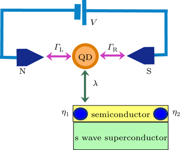
The N–QD–S system with coupled MBSs is illustrated in Fig. 1. A QD is connected with N and S leads. The QD can be fabricated by applying gate voltages on a two-dimensional electron gas.^[33] In addition, a semiconductor nanowire with strong Rashba interaction is subjected to a strong magnetic field B and adhere a proximity-induced s-wave superconductivity, then a pair of MBSs can form at the ends of the nanowire.^[2,7] In Fig. 1, the two MBSs are defined as η₁ and η₂. Here, we suppose that the QD is only connected to η₁ and the coupling strength is λ. We assume that the system under consideration is described by the following Hamiltonian:

Fig. 1.

	Figure Option ViewDownloadNew Window
	Fig. 1. Sketch of an N–QD–S system with coupled MBSs. A QD is connected with N and S leads. The QD is also connected to one end of a quantum wire on an s-wave supercunductor surface, which supports an MBS (blue dot) at each end. The two MBSs are defined as η1 and η2.

It is helpful to replace the Majorana fermion operators by ordinary fermion operators f and f^†, where f creates a fermion and f^† f = odd, even counts the parity of the MBS. In the new representation, we have and with {f,f^†} = 1. Accordingly, we can write H₀ in the form

The Fourier transformed retarded Green’s function of the system can be solved using Dyson's equation, where Σ^r is the self-energy matrix due to the tunneling coupling between the QD and the leads. In the 4 × 4 generalized Nambu-spin space, the free Green's function for the QD with the MBSs is given by

Once the retarded Green's functions are known, the electric current can be calculated using Eqs. (8) and (9). In this work, we only consider the Andreev transport for energies within the superconducting gap. Thus, the current amplitude corresponding to the contribution of quasiparticle tunneling is zero. In particular, the zero-bias AR conductance at zero temperature can be calculated as^[35]

In this section, we investigate the linear AR conductance at zero temperature in the N–QD–S system coupled with MBSs. In the numerical calculations discussed below, we consider a QD with only a single, spinless level of energy ɛ_d. The Fermi energy and the energy level of the QD are restricted to lie within the energy gap of the superconducting lead.

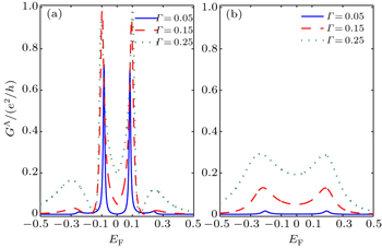
We first illustrate the AR conductance as a function of the Fermi energy in the N–QD–S system. For comparison, the results for the N–QD–S systems with and without coupled MBSs are respectively shown in Figs. 2(a) and 2(b). We set Δ = 1, ɛ_d = 0.2, ɛ_M = 0.1, and λ = 0.1. All parameters are expressed in units of the superconductor gap. For simplicity, we study only the symmetric case, and set Γ_L = Γ_R = Γ. In Figs. 2(a) and 2(b), the solid, dashed, and dotted lines denote Γ = 0.05, 0.15, and 0.25, respectively. It may be seen in Fig. 2(b) for the system without MBSs that the AR conductance curve exhibits two relatively weak peaks around the point E_F = ±0.2. The magnitudes of the peaks are much smaller than e²/h, though they increase as Γ increases. However, in the N–QD–S system with coupled MBSs, as shown in Fig. 2(a), the AR conductance curves exhibit double resonant peaks. The maximum conductance of the AR can reach as high as e²/h, and is only slightly affected by the coupling strengths of the QD to the leads. In addition, we obtain the symmetric line shape because the AR involves both the particle and hole degrees of freedom. From Fig. 2, we can see that in the N–QD–S system, even though the AR conductance curves generally exhibit weak peaks when no MBSs are present, for appropriate tunnel coupling with the normal and superconducting leads, the AR can be enhanced when coupling to the MBSs is incorporated. Next, we analyze the AR in the N–QD–S system with coupled MBSs in more detail.

Fig. 2.

	Figure Option ViewDownloadNew Window
	Fig. 2. AR conductance as a function of the Fermi energy in the N–QD–S systems (a) with and (b) without coupled MBSs. We set Δ = 1, ɛd = 0.2, ɛM = 0.1, and λ = 0.1. All parameters are expressed in units of the superconductor gap.

Figure 3 shows the AR conductance as a function of the Fermi energy in the N–QD–S system with coupled MBSs for different values of λ for the case of ɛ_M = 0 and ɛ_d = 0. From Fig. 3, we find several features of the AR conductance when only QD–MBS coupling is considered. First, in Fig. 3(a), for Γ = 0.01, we can clearly see four conductance peaks in each curve, located roughly symmetrically around the zero energy. In addition, the distance between the neighboring conductance peaks increases with increasing λ. When Γ increases from 0.01 to 0.1, as shown in Fig. 3(b), the conductance peaks are significantly suppressed, and one Fano line-shape appears in the AR conductance spectrum. These results can be easily understood. As shown in Fig. 1, the MBSs serve as a special electron reservoir with single energy mode. Electrons entering such a structure undergo phase randomization, thereby this tunneling channel is related to the dephasing mechanism. In practical terms, any decoherence is expected to suppressed the quantum features, therefore the stability of the Fano-type interference patterns can be regarded as a useful probe of an interplay between the coherence and incoherence tunneling channels. In this process, the AR conductance is always e²/2h at the point E_F = 0, showing the robust properties of the Majorana fermions.^[14]

Fig. 3.

	Figure Option ViewDownloadNew Window
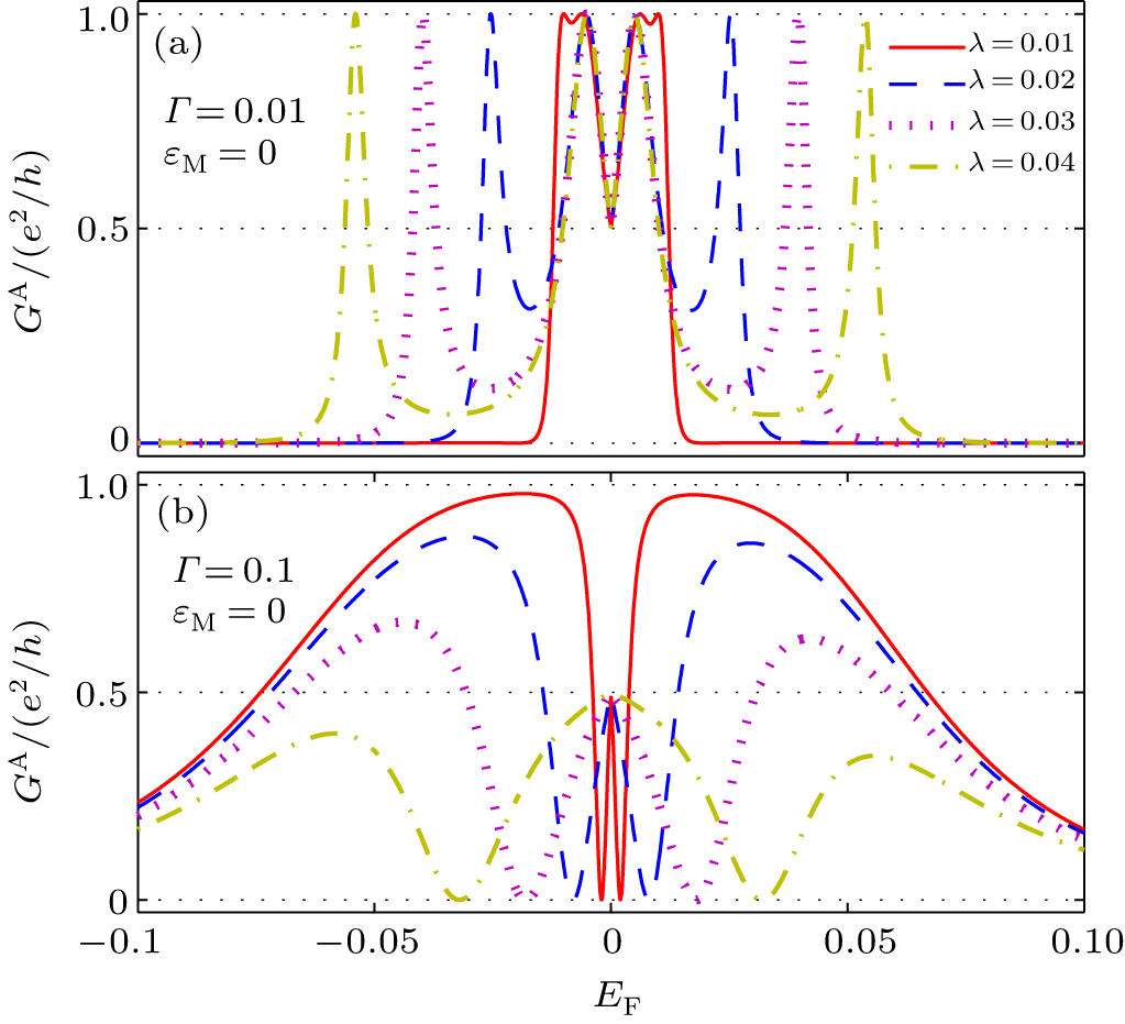
	Fig. 3. AR conductance as a function of the Fermi energy in the N-QD-S system with coupled MBSs for different values of λ when ɛd = 0 and ɛM = 0: (a) Γ = 0.01, (b) Γ = 0.1.

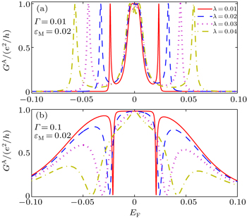
Figure 4 shows the AR conductance as a function of the Fermi energy in the presence of not only the QD–MBS coupling but also the coupling between the two MBSs. The zero energy conductance deviates from e²/2h once ɛ_M ≠ 0 as shown in Fig. 4. By a careful observation, one can also see that the coupling between the two MBSs widens the Fano resonance peak in Fig. 4(a) and the Fano antiresonance valley in Fig. 4(b). The N–QD–S structure with coupled MBSs provides two special transmission paths for the quantum interference. Therefore, the resonant channel for the Fano effect is simultaneously determined by both the weak QD–lead, QD–MBS coupling and the MBS–MBS coupling.

Fig. 4.

	Figure Option ViewDownloadNew Window
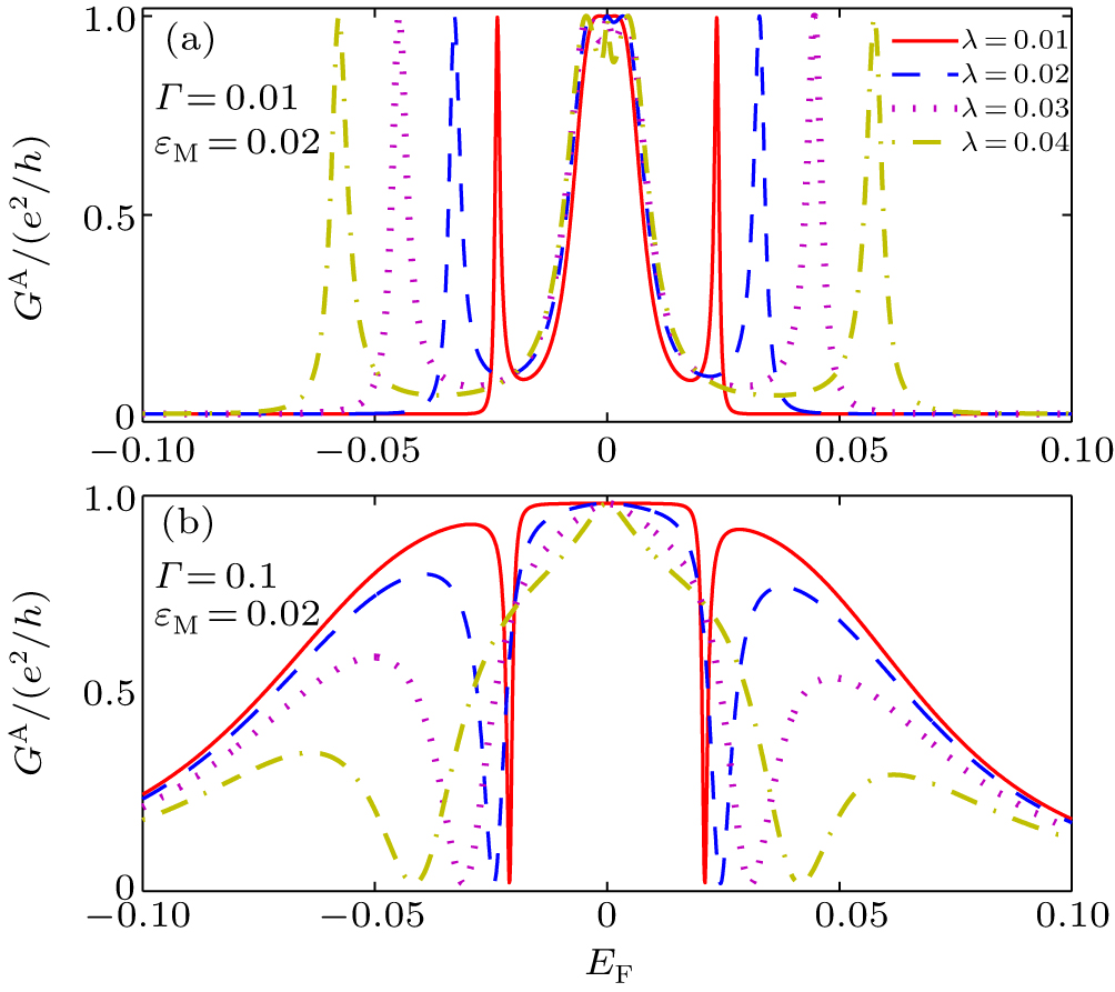
	Fig. 4. AR conductance as a function of the Fermi energy in the N–QD–S system with coupled MBSs for different values of λ when ɛd = 0 and ɛM = 0.02: (a) Γ = 0.01, (b) Γ = 0.1.

Next, in Fig. 5, we illustrate the influence of changes in the MBS–MBS coupling on the AR conductance. In Fig. 5(a), when Γ = 0.01, one can see that the resonant peaks shift away from the zero Fermi energy point. In addition, one can see from Fig. 5(b) that when Γ = 0.1, the resonant line-shapes are greatly modified as ɛ_M increases. For example, in Fig. 5(b), the solid red line, ɛ_M = 0.02, is a small antiresonance with a peak at E_F = 0. With ɛ_M increasing to ɛ_M = 0.06 (see the blue dashed line in Fig. 5(b)), the original primary resonant peak becomes wider and the second peaks develop into a Fano line shape.

Fig. 5.

	Figure Option ViewDownloadNew Window
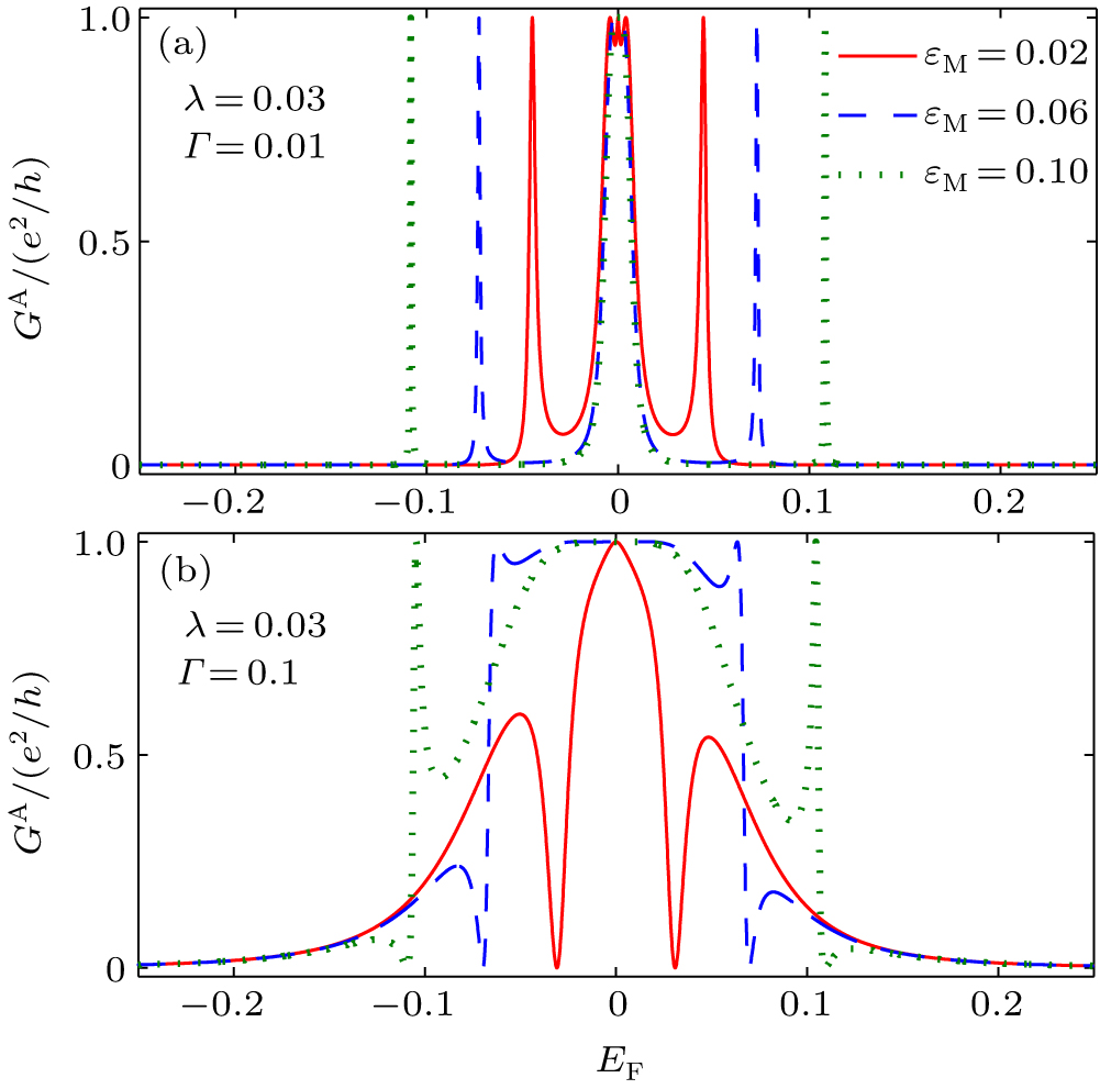
	Fig. 5. AR conductance as a function of the Fermi energy in the N–QD–S system with coupled MBSs for different values of ɛM when ɛd = 0 and λ = 0.03: (a) Γ = 0.01, (b) Γ = 0.1.

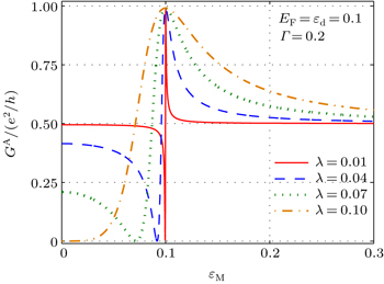
In order to obtain a better understanding of the above behaviors, in the following, we focus on under what conditions the Fano resonant AR might appear. In Fig. 6, we show the AR conductance at E_F = ɛ_d = 0.1 as a function of ɛ_M with different values of the QD–η₁ coupling λ for fixed Γ = 0.2. We can see that with these parameters, the AR conductance changes with ɛ_M. Obviously, there is a critical value ɛ_Mc. When ɛ_M < ɛ_Mc, the AR conductance decreases with increasing ɛ_M. When ɛ_M > ɛ_Mc, the AR conductance quickly increases from zero to the maximum e²/h, and then decreases to e²/2h slowly as ɛ_M increases further. The critical point is dependent on both λ and Γ. For fixed Γ, the critical value ɛ_Mc increases with decreasing λ. When ɛ_M = 0.1, which just equals to the energy level of the QD, the resonant AR occurs quickly and gives the maximum AR conductance; when ɛ_M deviates from this point, the AR conductance quickly decreases to e²/2h.

Fig. 6.

	Figure Option ViewDownloadNew Window
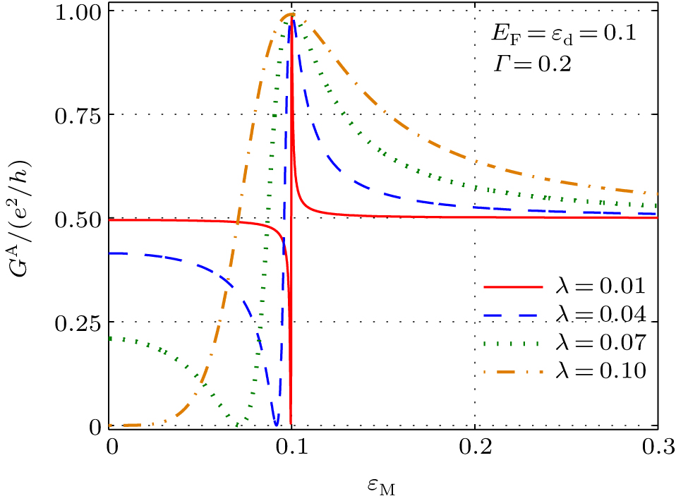
	Fig. 6. AR conductance as a function of ɛM in the N–QD–S system with coupled MBSs for different values of λ when EF = ɛd = 0.1 and Γ = 0.2.

We also calculate the AR conductance as a function of λ for different values of ɛ_M for the case of Γ = 0.2 and E_F = ɛ_d = 0.1. The results are shown in Fig. 7. When ɛ_M = ɛ_d (see the black dot-dashed line in Fig. 7), an intense resonance occurs, and the AR conductance increases quickly from the initial value e²/2h to the maximum e²/h. When ɛ_M > ɛ_d, G^A increases gradually from e²/2h to e²/h with increasing λ. However, for ɛ_M < ɛ_d, there is a critical value of λ, λ_c, corresponding to G^A = 0. When λ < λ_c, G^A decreases from e²/2h to zero with increasing λ. Once λ > λ_c, G^A increases gradually from zero to its maximum and remains at the maximum value with a further increase in λ.

Fig. 7.

	Figure Option ViewDownloadNew Window
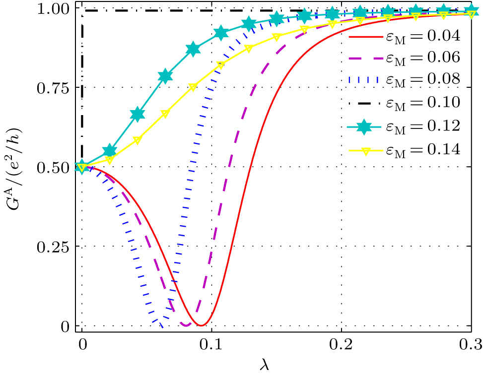
	Fig. 7. AR conductance as a function of λ in the N–QD–S system with coupled MBSs for values of ɛM when EF = ɛd = 0.1 and Γ = 0.2.

We have studied the AR in an N–QD–S system coupled with MBSs. We found that for appropriate tunnel coupling with the normal and superconducting leads, the AR is enhanced by the MBSs. For a given Fermi energy, one can tune the gate voltage to obtain a primary resonant state. One can then change the coupling strength between the QD and the MBS η₁ or between the two MBSs to obtain a Fano resonance. The AR conductance is always e²/2h at the zero energy point when only QD–MBSs coupling is considered, showing the robust properties of the Majorana fermions. In addition, with strong QD–MBS coupling, the resonant AR can occur even in the absence of coupling between the two MBSs. When the MBS–MBS coupling roughly equals to the QD energy level, the resonant AR can also occur even with very weak QD–MBS coupling. We also found that an AR antiresonance appears when the QD energy level approximately equals to the sum of the QD–MBS coupling and the MBS–MBS coupling. Based on all the numerical results, we propose that such a system may be a candidate for detecting the MBSs. Furthermore, these results will be helpful for understanding the quantum interference in MBS-assisted AR and may find significant applications, especially in quantum computation.