Epidemic spreading has been a challenging problem for a long time as it usually causes major public health threats owing to their potential mortalities and substantial economic impacts. Its recent examples are the outbreaks of global infectious diseases including SARS (Severe Acute Respiratory Syndrome), H1N1 (Swine Influenza), H5H1 (Avian Influenza), and Ebola, etc. To understand how epidemics spread in a system, which is a crucial step to preventing and controlling outbreaks, several models have been proposed such as the susceptible-infected-susceptible (SIS) and susceptible-infected-refractory (SIR) models, etc.,^[1] where S, I, and R represent the susceptible, infected, and refractory individuals, respectively. Based on these models, it is revealed that the epidemic can be spread out only when its infection rate is greater than a threshold.

The study of epidemics has been a very hot research topic in recent decades, due to the fast progress in network science.^[2,3] It is revealed that the stabilized epidemic depends on many factors such as the network structure, adopted immunization, received information, and chosen traveling, etc. For example, it was found that the epidemic spreading on scale-free networks has no epidemic threshold in the thermodynamic limit.^[4–11] Different approaches of immunization will result in different effects of controlling an epidemic, such as the targeted immunization^[12–14] and acquaintance immunization,^[15,16] etc. Received information will make individuals take self-protective actions to protect themselves.^[17–21] Epidemic spreading on one layer will asymmetrically interact with the communication on another layer.^[22,23] Objective traveling of choosing the shortest path will accelerate the epidemic spreading,^[24–28] in contrast to the random diffusion model where individuals randomly choose one of its neighboring nodes for diffusion.^[29–33]

Currently, the study of epidemics is focusing on the multi-layered networks where a variety of dynamics can be investigated.^[34–36] A great deal ofattention has been paid to the case of multiple pathogens, where two or more diseases spread in the same population and each person can be infected by two or more of them.^[37–42] In fact, this case is more realistic. For example, it was revealed that the persons infected by HIV have a higher risk to be infected by other pathogens, including hepatitis, tuberculosis, and malaria.^[43,44] It was also found that the incidence of tuberculosis was increased during the 1918–1919 Spanish flu.^[45,46] These evidences show that infection by one pathogen can effectively influence the infection process by the other pathogen, which may be either competitive or cooperative for the same population of hosts. Focusing on the two-pathogen scenario, it has been found that the onset of a disease’s outbreak is conditioned to the prevalence levels of the other disease. For the case of competitive (cooperative) interaction between two pathogens, the presence of one pathogen makes the other less (more) likely to spread.^{[37,42,44,47–50]}

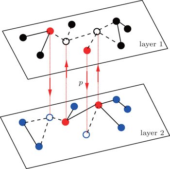
A typical but interesting case of multiple pathogens is sexually transmitted diseases, which can propagate in both heterosexual and homosexual networks of sexual contacts.^[51,52] This problem has been recently considered by Sanz et al.^[53] and our team.^[54] Sanz et al. thoroughly studied extensions of the SIS and SIR models, based on the condition of constant infection rates. While we presented a unified framework to study both the cooperative and competitive interactions between two pathogens in multiplex networks, based on a new concept of a state-dependent infectious rate.^[54] However, all these considerations ignore the effect of bisexual men, which is evidenced to increase the AIDS-related risk.^[55,56] A study on the number of partners among U.S. bisexual men shows that bisexual men are the medium to connect the pathogens in the network of heterosexual men with the pathogens in the network of homosexual men.^[55–59] Based on these evidences, we here study this problem by focusing on the role of bisexual individuals, i.e., connecting the heterosexual network and homosexual network. Thus, we present a two-layered network model without fixed links between the two layers, but with dynamic propagators to connect the two layers. This model is not only limited for sexually transmitted diseases, but also for other pathogens caused by traveling between different cities. In detail, we let each layer have a distinct pathogen and let the propagators have a chance to jump between the two layers at each time step, see Fig. 1. That is, without the propagators, the two layers will be completely separated. In this way, the coupling between the two layers is not by some persistent links as in each layer but by a new type of impulsive links, i.e., jumping. To the best of our knowledge, this is the first model to consider impulsive links. By this model we show that (i) the propagators take the key role to transmit pathogens from one layer to the other, which significantly influences stabilized epidemics; (ii) the epidemic thresholds will be changed by the propagators; and (iii) a reverse-feeding effect can be expected when the infective rate is smaller than its threshold of isolated spreading. A theoretical analysis is presented to explain the numerical results.

Fig. 1.

Figure Option ViewDownloadNew Window

Fig. 1. Schematic figure of sexually transmitted diseases on a two-layered network where the up and down layers represent the networks of homosexual and heterosexual individuals, respectively, and are connected by the impulsive jumping of the bisexual individuals, called propagators. The “black” nodes represent the homosexual individuals, “blue” nodes the heterosexual individuals, the “red” nodes the bisexual individuals, and the “hole” nodes are for the jumping. The solid lines represent the active links while the dashed lines denote the inactive links. Each bisexual individual has a probability p to jump to its corresponding “hole” node at each time step.

The rest of this paper is organized as follows. In Section 2, we introduce the model to study the effect of the propagators. Then in Section 3, we make numerical simulations to show how the propagators influence the spreading of the two pathogens, especially the epidemic thresholds. After that, we give a brief theoretical analysis to explain the numerical results in Section 4. Finally, we give discussions and conclusions in Section 5.

Figure 1 shows the schematic figure of our model. For simplicity, the up (“layer 1”) and down (“layer 2”) layers are considered to be two independent random Erdös-Rényi networks^[2] with sizes N₁ and N₂ and average degrees ⟨k₁⟩ and ⟨k₂⟩, respectively. We assume that there are totally m propagators in the network and they are initially half in the up layer and the other in the down layer. The propagators have a double identity. They will behave only as homosexual (heterosexual) people when they are at the homosexual (heterosexual) layer. At each time step, every propagator will have a probability p to jump from its layer to the other layer. To smoothly implement this jumping process, we randomly choose m nodes from each layer and let them be fixed as the host nodes for the propagators. When the propagators are staying at these host nodes, their connections to neighbors will be active (see the “red” nodes in Fig. 1); otherwise, their connections to neighbors will be inactive (see the “empty” nodes in Fig. 1). In this sense, we will initially choose m/2 occupied nodes for the propagators and m/2 “hole” nodes at each layer. We will always have N₁ − m non-jumping nodes at the up layer and N₂ − m non-jumping nodes at the down layer. We let a propagator from one layer and a hole node from the other layer form a corresponding pair of nodes, see those pairs of nodes connected by the dotted “red” lines between the two layers in Fig. 1 with the “arrow” being the jumping direction. That is, each propagator can jump only to its corresponding “hole” node.

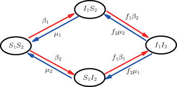
Then, we assume two pathogens in the network, i.e., pathogen-1 on the up layer and pathogen-2 on the down layer. Without propagators, the two pathogens will independently spread on their individual layers, respectively. With propagators, the two pathogens will spread on both the two layers. Therefore, there will be a dynamical interaction between the two pathogens once they spread to the same nodes. To understand how this dynamical interaction influences epidemic spreading, we here take the susceptible-infected-susceptible (SIS) model for both the two pathogens as an example. In the SIS model, a susceptible node may be infected by an infected neighbor at rate β when it contacts one infected node. At the same time, each infected node will become susceptible again at rate μ at each time step.^{[1,4,5,7,60–63]} In the case of complex networks, a susceptible node may have k_inf infected neighbors, thus it will become infected with probability 1 − (1 − β)^k_inf. While the present case is more complicated as it has two interacting pathogens. To describe it, we let the set (S₁, I₁) represent pathogen-1 and the set (S₂, I₂) represent pathogen-2. In this case, a node will have 4 states: S₁S₂ — the node is susceptible to both pathogen-1 and pathogen-2; I₁S₂ — the node is infected by the first pathogen-1 but susceptible to pathogen-2; S₁I₂ — the node is susceptible to the first pathogen-1 but infected by the second pathogen-2; and I₁I₂ — the node is infected by both pathogen-1 and pathogen-2.^[53,54]

Figure 2 shows the schematic illustration of the transition in the four status of a node, where the transition between S₁S₂ and I₁I₂ is ignored as a person will usually not be infected by two pathogens at exactly the same time. Let β₁ (β₂) and μ₁ (μ₂) be the infective and recovery rates of pathogen-1 (pathogen-2), respectively. Then, an S₁S₂ node will be infected into an I₁S₂ status by a probability 1 − (1 − β₁)^k_inf1, where k_inf1 is the number of its total infected neighbors with either status I₁S₂ or status I₁I₂. At the same time, each I₁S₂ node will recover to the S₁S₂ status by a probability μ₁. Similarly, an S₁S₂ node will become the S₁I₂ status by a probability 1 − (1 − β₂)^k_inf2, where k_inf2 is the number of its total infected neighbors with either status S₁I₂ or status I₁I₂. At the same time, each S₁I₂ node will recover to the S₁S₂ status by a probability μ₂.

Fig. 2.

	Figure Option ViewDownloadNew Window
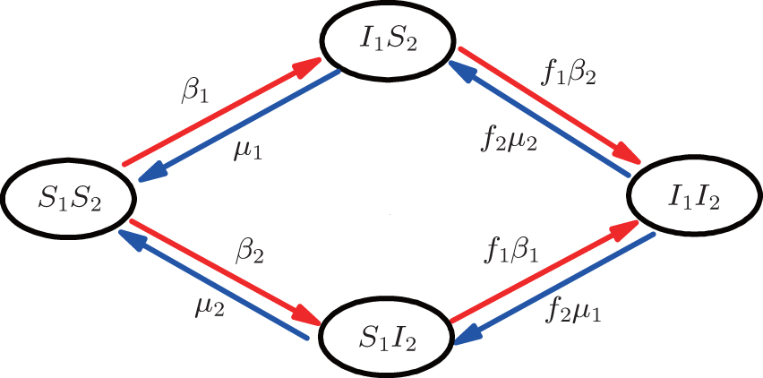
	Fig. 2. Schematic illustration of the transition in the four status of a node, see the text for a detailed explanation.

For an infected node, its secondary infection by another pathogen will be different from its first infection. It has been revealed that an infection by malaria is shown to increase an individual’s attractiveness to mosquitos,^[64] which in turn may increase the chance to be infected by other strains. Generally, an infected person will become weakened and thus can be more likely to be attacked by another pathogen, which corresponds to the case of cooperation between two pathogens. On the other hand, when an infected person takes medicine, he will be less likely to get the other, which corresponds to the case of competition between two pathogens. We here introduce a factor to reflect this kind of cooperation or competition. In detail, we let f₁ be the infection factor and f₂ be the recovery factor. Thus, an I₁S₂ node will become the I₁I₂ status by a probability 1 − (1 − f₁β₂)^k_inf2. At the same time, each I₁I₂ node will recover to the S₁I₂ status by a probability f₂μ₂. Similarly, an S₁I₂ node will become the I₁I₂ status by a probability 1 − (1 − f₁β₁)^k_inf1. At the same time, each I₁I₂ node will recover to the S₁I₂ status by a probability f₂μ₁.

We are here mainly focused on how the impulsive jumping between the two networks influences the epidemic spreading, as it is what happens in reality and has not been paid attention so far. It is well known that the network topology will seriously influence the epidemic spreading.^[2,3] To reduce the influence from the aspect of network topology, we limit the jumping probability to a very small range, i.e., p ≪ 1. In this condition, the main influence between the two layers will come from the effect of jumping. We will use the random Erdös–Rényi networks as an example, as it is a good candidate for the mean-field approach. We find that the obtained results also work for other networks such as the scale-free networks.

In numerical simulations, we first construct two independent random Erdös–Rényi networks^[2] as the up and down layers of Fig. 1, respectively. Notice that there are fewer homosexual people than heterosexual people, implying that the two networks in Fig. 1 will have different sizes. Thus, as an example, we here let the up network have N₁ = 1000 nodes and the down network have N₂ = 4000 nodes. To reflect the different ways of communication in the homosexual and heterosexual communities, we let the average degrees of the up network be ⟨k₁₀⟩ = 8 and that of the down network be ⟨k₂₀⟩ = 3. We let the number of total propagators be m = 400, i.e., there are initially m/2 = 200 propagators in each of the up and down layers. The non-jumping nodes will be 600 in the up layer and 3600 in the down layer. When the jumping probability p is zero, the up and down networks become independent. Notice that the links of the hole nodes in Fig. 1 are inactive. When the hole nodes are not neighboring each other, we have ⟨k₁₀⟩ m/2 inactive links in the up network and ⟨k₂₀⟩ m/2 inactive links in the down network. In general, it is possible for the hole nodes to also be neighbors of each other, indicating that the average degree of the up layer ⟨k₁⟩ will be less than ⟨k₁₀⟩ but greater than (N₁ ⟨k₁₀⟩ − 2 ⟨k₁₀⟩ m/2)/(N₁−m/2) = ⟨k₁₀⟩ (N₁ − m)/(N₁ − m/2). Similarly, the average degree of the down layer ⟨k₂⟩ will be less than ⟨k₂₀⟩ but greater than ⟨k₂₀⟩ (N₂ − m)/(N₂ − m/2). When the hole nodes are non-neighbors, we have ⟨k₁⟩ = ⟨k₁₀⟩ (N₁ − m)/(N₁ − m/2) = 6 and ⟨k₂⟩ = ⟨k₂₀⟩ (N₂ − m)/(N₂ − m/2) ≈ 2.84. For a homogeneous random network, we have the critical infection rate β_c = μ/⟨k⟩.^[65,66] Taking μ₁ = μ₂ = 0.01 as an example, we will have the thresholds β_1c0 ≈ μ/⟨k₁⟩ ≈ 0.00167 for the up layer and β_2c0 ≈ μ/⟨k₂⟩ ≈ 0.00352 for the down layer when the two layers are isolated with p = 0.

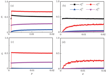
We now consider epidemic spreading by fixing μ₁ = μ₂ = 0.01 in this paper. We choose the factors f₁ = 1.4 and f₂ = 1, unless otherwise specified. Initially, we randomly choose a few nodes of the up (down) layer of Fig. 1 to be the infected seeds of pathogen-1 (pathogen-2). Then, we let the system evolve to a stabilized state and measure the density of infected nodes ρ_I, which includes both the first infection I₁S₂ or S₁I₂ and the secondary infection I₁I₂. We let , (, ) represent the densities of pathogen-1 and pathogen-2 in the up (down) layer, respectively, which exclude the hole nodes. Figure 3 shows the dependence of ρ_I on the jumping probability p with the “squares”, “circles”, “uptriangles”, and “downtriangles” being , , , and , respectively, where panel (a) represents the case of β₁ = 0.003 and β₂ = 0.005, (b) the case of β₁ = 0.003 and β₂ = 0.003, (c) the case of β₁ = 0.0014 and β₂ = 0.005, and (d) the case of β₁ = 0.0014 and β₂ = 0.003. The parameters in Fig. 3 are chosen for four typical situations, i.e. β₁ > β_1c0 and β₂ > β_2c0 in panel (a), β₁ > β_1c0 and β₂ < β_2c0 in panel (b), β₁ < β_1c0 and β₂ > β_2c0 in panel (c), and β₁ < β_1c0 and β_1c0 < β₂ < β_2c0 in panel (d). A common point in the four panels of Fig. 3 is that when p = 0, there is at most one pathogen of ρ_I > 0 for each layer, confirming the independence of the two layers at p = 0.

Fig. 3.

Figure Option ViewDownloadNew Window

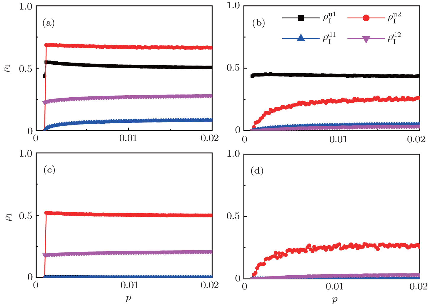
Fig. 3. Dependence of ρI on the jumping probability p with the “squares”, “circles”, “uptriangles”, and “downtriangles” being , , , and , respectively, where panel (a) represents the case of β1 = 0.003 > β1c0 and β2 = 0.005 > β2c0, (b) the case of β1 = 0.003 > β1c0 and β2 = 0.003 < β2c0, (c) the case of β1 = 0.0014 < β1c0 and β2 = 0.005 > β2c0, and (d) the case of β1 = 0.0014 < β1c0 and β2 = 0.003 < β2c0 but with β2 > β1c0. The results are averaged over 1000 realizations.

The chosen values of β₁ > β_1c0 and β₂ > β_2c0 in Fig. 3(a) guarantee that both pathogen-1 and pathogen-2 can spread in their host layers when p = 0. When p > 0, the infected seeds of pathogen-1 (pathogen-2) will be transmitted to the down (up) layer and then cause its spreading there. In the up layer of the case of Fig. 3(a), both β₁ and β₂ are greater than β_1c0 and thus they can both spread out, provided that the propagators can transmit the infected seeds of pathogen-2 from the down layer to the up layer. The final and are mainly determined by β₁ − β_1c0 and β₂ − β_1c0, which results in their approximate constant values in Fig. 3(a). While in the down layer, we have β₁ < β_2c0, thus the seeds of pathogen-1 cannot spread out but can only stay there for a transient time. As the recovery rate μ₂ = 0.01 < 1, a transmitted seed of pathogen-1 will keep its status for some time steps before it jumps back to the up layer. In this sense, p > 0 will provide persistent jumping seeds of pathogen-1 into the down layer and thus the value of will be proportional to p. On the other hand, for an individual seed, its effect of epidemic spreading depends not only on the jumping speed but also on the contacting time,^[25] resulting in a nonlinear dependence of on p, as in Fig. 3(a). Figures 3(b) and 3(c) can be similarly explained. Comparing the corresponding values of in Figs. 3(c) and 3(a), we see that is about 0.5 in panel (c) and 0.7 in panel (a), indicating a significant difference. The reason is that there is no interaction between the two pathogens in Fig. 3(c) with but with interaction in Fig. 3(a) with , indicating that the interaction has significantly influenced the spreading of the two pathogens.

We now turn to Fig. 3(d) with both β₁ < β_1c0 and β₂ < β_2c0. When p = 0, there are neither nonzero pathogen-1 nor nonzero pathogen-2 in the system. However, p > 0 induces an interesting phenomenon that and are both nonzero! This phenomenon can be explained as follows. The initial seeds of pathogen-2 will spread on the down layer for some time before its death. During this time period, the jumping propagators will have the chance to bring pathogen-2 into the up layer. As we have β₂ > β_1c0, the transmitted seeds of pathogen-2 will spread out on the up layer. Then, the propagators will send pathogen-2 back to the down layer and thus sustain the nonzero there, resulting in an interesting “reverse-feeding” phenomenon.

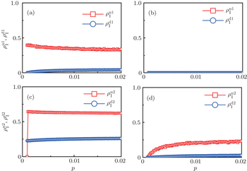
To understand the underlying mechanism of the nonlinear dependence of ρ_I on p in the four panels of Fig. 3, we divide its complicated dynamics into two aspects, i.e., the structure and mutual influence of two pathogens. Firstly, we focus on the aspect of structure, i.e., different average degrees between the up and down layers. To clearly see its effect, we consider the case of only one pathogen in the network. Figures 4(a) and 4(b) show the results of β₂ = 0, where panel (a) represents the case of β₁ = 0.003 > β_1c0 and panel (b) the case of β₁ = 0.0014 < β_1c0. From Fig. 4(a) we see that with the increase of p, is slightly decreased while increases from zero gradually. This result can be explained as follows. As β₁ = 0.003 < β_2c0, the epidemic cannot spread out at the down layer, indicating that is mainly obtained by the jumping process. In this sense, the increase of p will result in an increase of . At the same time, the jumping will make be slightly decreased. From Fig. 4(b) we see that both and are zero, which can be easily understood by β₁ = 0.0014 being smaller than both β_1c0 and β_2c0.

Fig. 4.

Figure Option ViewDownloadNew Window

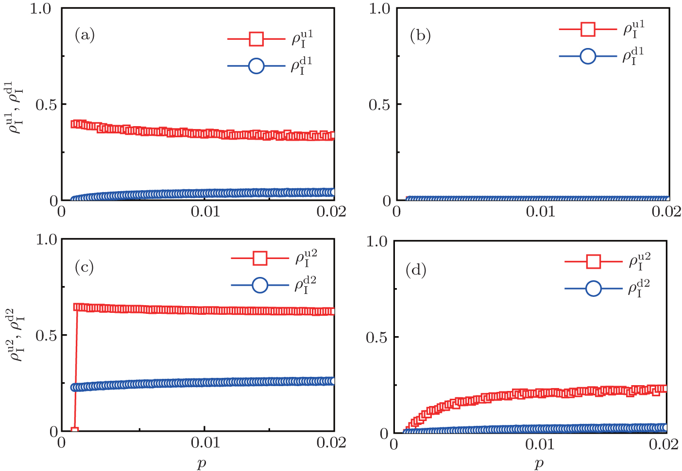
Fig. 4. Influence of structure difference of the two layers on epidemic spreading. Panels (a) and (b) show the case of β2 = 0, where and represent the infected densities of pathogen-1 at the up and down layers, respectively. The parameter β1 is chosen as β1 = 0.003 > β1c0 in panel (a) and β1 = 0.0014 < β1c0 in panel (b). Panels (c) and (d) show the case of β1 = 0, where and represent the infected densities of pathogen-2 at the up and down layers, respectively. The parameter β2 is chosen as β2 = 0.005 > β2c0 in panel (c) and β2 = 0.003 < β2c0 in panel (d).

Figure 4(c) and 4(d) show the results of β₁ = 0, where panel (c) represents the case of β₁ = 0.005 > β_2c0 and (d) the case of β₂ = 0.003 < β_2c0. From Fig. 4(c) we see that with the increase of p, both and are approximately constants. This result can be explained as follows. As β₂ = 0.005 is greater than both β_2c0 and β_1c0, the epidemic can spread out at both the up and down layers. In this situation, will be determined by β₂–β_1c0 and will be determined by β₂ − β_2c0. Thus, the influence of p can be ignored. Figure 4(d) shows a completely different case where both and increase with the increase of p but with . The reason is that β₂ = 0.003 is smaller than β_2c0 but greater than β_1c0. The condition of β₂ < β_2c0 will make the epidemic not be spread out, indicating no epidemic at both the up and down layers when p = 0. However, when p > 0, it is possible for pathogen-2 to be transmitted to the up layer by the propagators. Once it happens, pathogen-2 will spread out at the up layer because β₂ > β_1c0. Then the propagator will bring the infected ones back to the down layer and thus result in a sustained , i.e. “reverse-feeding” phenomenon, indicating that the effect of reverse-feeding is mainly from the difference of thresholds between β_2c0 and β_1c0 caused by the different average degrees between the up and down layers.

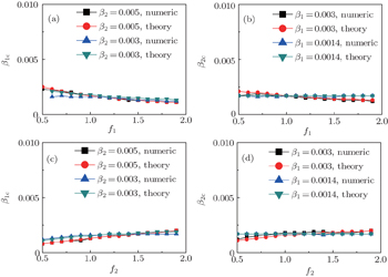
Secondly, we consider the aspect of mutual influence of two pathogens, where f₁ and f₂ are the two key parameters to determine the feature of interaction, i.e. cooperation or competition. To clearly see its effect, we focus on the influence of f₁ and f₂ on the epidemic thresholds. We let β_1c and β_2c be the epidemic thresholds of the up and down layers with p > 0, respectively. We first check the effect of f₁ by fixing f₂ = 1 and p = 0.005. Figure 5(a) shows how β_1c depends on f₁ where the “squares” and “uptriangles” represent the cases of β₂ = 0.005 and 0.003, respectively. From Fig. 5(a) we see that β_1c decreases with the increase of f₁ for the two cases but is faster in the case of β₂ = 0.005 than that of β₂ = 0.003. This result can be understood as follows. As β₂ = 0.005 is greater than both β_1c0 and β_2c0, pathogen-2 can spread out in both the up and down layers, implying an interaction between the two pathogens in the up layer. Notice that an increase of f₁ means the enhanced cooperation between the two pathogens. Therefore, the increase of f₁ will result in an enhanced spreading of and thus a decreased β_1c on f₁. While in the case of β₂ = 0.003, its will be much smaller than that of β₂ = 0.005, indicating its interaction with will be much weaker than that of β₂ = 0.005 and thus will result in a slower decreased β_1c on f₁.

Figure 5(b) shows how β_2c depends on f₁ where the “squares” and “uptriangles” represent the cases of β₁ = 0.003 and 0.0014, respectively. From Fig. 5(b) we see that β_2c decreases with the increase of f₁ for the case of β₁ = 0.003 but keeps a constant for the case of β₁ = 0.0014. This result is easy to understand. As β₁ = 0.003 is greater than β_1c0 but smaller than β_2c0, there will be a small quantity of at the down layer by the jumping process. Its interaction with will enhance the spread of pathogen-2 and thus result in a decreased β_2c on f₁. While β₁ = 0.0014 is smaller than both β_1c0 and β_2c0, there will be no and thus no interaction with , resulting in a constant β_2c.

Fig. 5.

Figure Option ViewDownloadNew Window

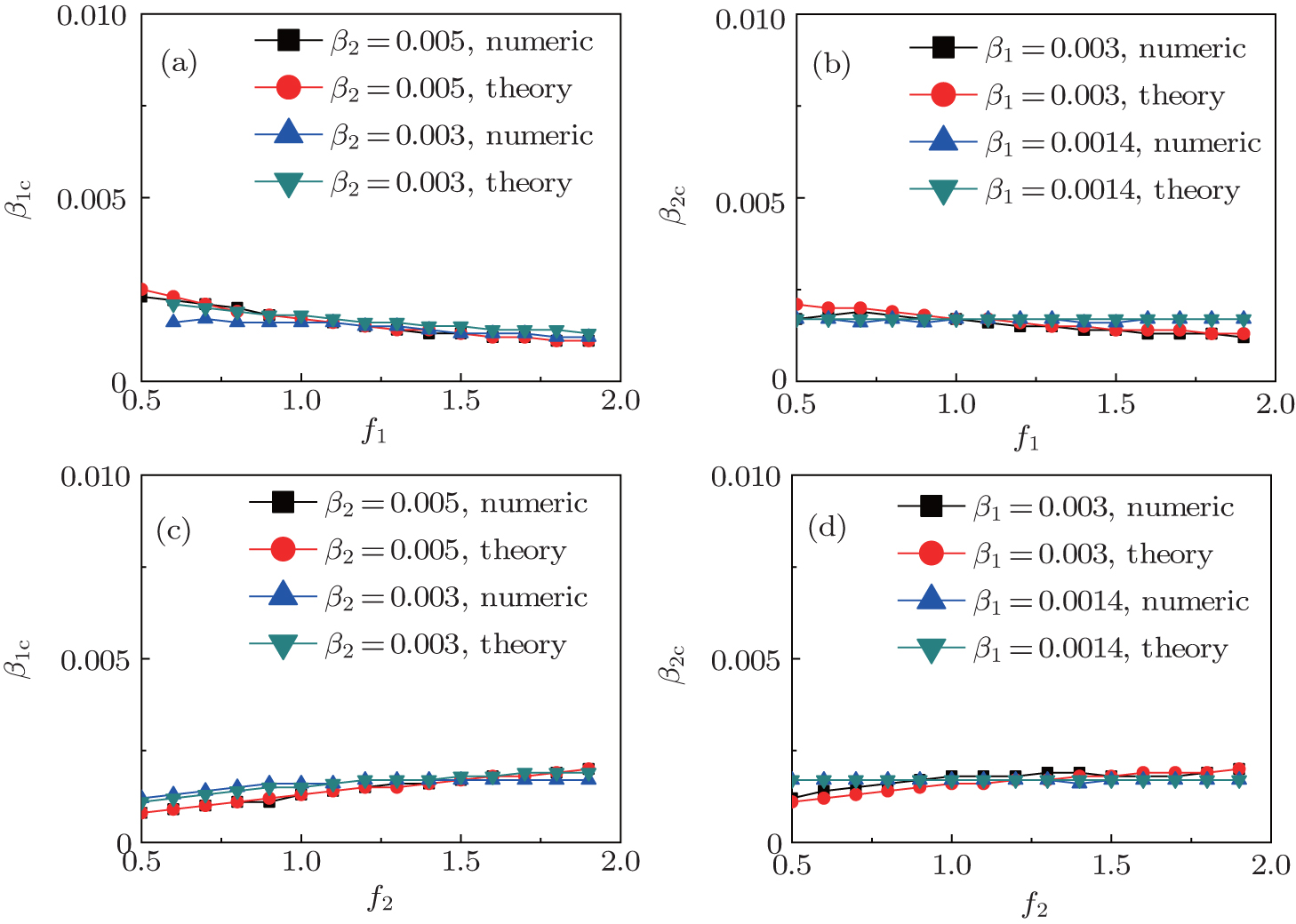
Fig. 5. Influence of f1 and f2 on the epidemic thresholds β1c and β2c with fixed p = 0.005, where the “squares” and “uptriangles” represent the numerical simulations and “circles” and “downtriangles” represent the corresponding theoretical results from Eqs. (2)–(5). (a) β1c versus f1 with f2 = 1, where the “squares” and “uptriangles” represent the cases of β2 = 0.005 and 0.003, respectively. (b) β2c versus f1 with f2 = 1, where the “squares” and “uptriangles” represent the cases of β1 = 0.003 and 0.0014, respectively. (c) β1c versus f2 with f1 = 1, where the “squares” and “uptriangles” represent the cases of β2 = 0.005 and 0.003, respectively. (d) β2c versus f2 with f1 = 1, where the “squares” and “uptriangles” represent the cases of β1 = 0.003 and 0.0014, respectively. The results are averaged over 1000 realizations.

We now turn to check the effect of f₂ by fixing f₁ = 1 and p = 0.005. Figure 5(c) shows how β_1c depends on f₂ where the “squares” and “uptriangles” represent the cases of β₂ = 0.005 and 0.003, respectively. Figure 5(d) shows how β_2c depends on f₂ where the “squares” and “uptriangles” represent the cases of β₁ = 0.003 and 0.0014, respectively. Comparing Figs. 5(c) and 5(d) with Figs. 5(a) and 5(b), respectively, we see that their dependence on f₁ and f₂ is the opposite, confirming the role of the infection factor f₁ and the role of the recovery factor f₂.

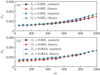
Finally, we discuss how the parameter m influences the thresholds β_1c and β_2c. We fix the total numbers of nodes N₁ and N₂ and let p = 0.005, f₁ = 1.4, and f₂ = 1. When m increases, the non-jumping nodes in both the up and down layers will decrease by N₁ − m and N₂ − m, respectively, which results in the decrease of ⟨k₁⟩ and ⟨k₂⟩ and then the increase of β_1c and β_2c. Figure 6 shows the results where the “squares” and “uptriangles” in panel (a) represent the cases of β₂ = 0.005 and 0.003, respectively, and the “squares” and “uptriangles” in panel (b) represent the cases of β₁ = 0.003 and 0.0014, respectively. From Fig. 6(a) we see that the line with “squares” is smaller than that of “uptriangles”, implying that a larger β₂ has a stronger influence on the threshold β_1c. We see the same result in Fig. 6(b), indicating that a larger β₁ also has a stronger influence on the threshold β_2c.

Fig. 6.

Figure Option ViewDownloadNew Window

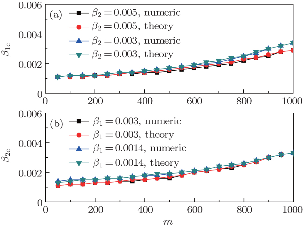
Fig. 6. Dependence of the thresholds β1c and β2c on m with fixed p = 0.005, f1 = 1.4, and f2 = 1, where the results are averaged over 1000 realizations. (a) β1c versus m where the “squares” and “uptriangles” represent the cases of β2 = 0.005 and 0.003, respectively, and “circles” and “downtriangles” represent the corresponding theoretical results, respectively. (b) β2c versus m where the “squares” and “uptriangles” represent the cases of β1 = 0.003 and 0.0014, respectively, and “circles” and “downtriangles” represent the corresponding theoretical results, respectively.

We now conduct a theoretical analysis on the above numerical simulations. For convenience, we introduce , , , and to represent the four densities of status [SS, IS, SI, II] in the up layer. Similarly, we let , , , and to represent the four densities of status [SS, IS, SI, II] in the down layer. Thus, we have

We divide the dynamics process into two steps, i.e. reaction and jumping. For the former, we use the mean-field approach to figure out the densities ρ_SS, ρ_IS, ρ_SI, and ρ_II. According to Fig. 2, the evolution equations of the two epidemics in the up layer can be given as

In the jumping process, we have

The nonlinear algebraic equations (7) and (8) are our final results. To compare them with the obtained numerical results, we first consider the specific case of one pathogen such as β₂ = 0. From Eq. (6) we have

For a general solution of the nonlinear algebraic equations (7) and (8), we have two ways to obtain it. The first one is to calculate the fixed point of Eqs. (7) and (8) by the Newton–Raphson method or other similar ones. The second one will start with the initial conditions of , , , , and , , , , and then iterate Eqs. (2)–(5) until a steady state is reached. We here use the second way to get the solution. For each set of parameters chosen, we first figure out the values of ⟨k₁⟩ and ⟨k₂⟩ by counting the total links of the active nodes and making average on time. Then, we substitute them into Eqs. (2)–(5) and focus on the thresholds β_1c and β_2c. The “circles” and “down triangles” in Fig. 5(a)–5(d) represent the theoretical results. Comparing them with the corresponding numerical results, we see that they are consistent with each other very well. After the same process, we can obtain β_1c and β_2c for different m, see the “circles” and “downtriangles” in Figs. 6(a) and 6(b). Clearly, they are also consistent with the corresponding numerical results very well.

The present study is for the interaction between two SIS pathogens, but it can be easily extended to other cases such as two SIR pathogens, one SIS and one SIR pathogens, or even more than two pathogens. Further, our model can also be extended to the case of traveling between different cities where the travelers take the role of propagators. Although this work is the primary try to consider the role of propagators, its further studies may provide guiding to human mobility patterns and thus may help public health services understand and control human infectious diseases.

In conclusion, we have presented a model of two interactive pathogens in two-layered networks where the connection between the two layers is implemented by a small fraction of propagators. We interestingly find a reverse-feeding phenomenon that the stabilized epidemic spreading on one layer can be sustained by the persistent jumping of propagators from the other layer. When focusing on the thresholds with p > 0, we find that the jumping and the mutual interaction between the two pathogens will reduce both β_c1 and β_c2. We further show that the reduced epidemic thresholds come mainly from two aspects. One is the different average degrees between the two layers. The other is the modified immune system of the secondary infection, which can be characterized by the factors of f₁ and f₂. A mean-field theory is provided to explain the underlying mechanism of the epidemic spreading in the model. This work provides significant implications for controlling epidemic spreading in realistic cases.