All-metal vibration insulators have high strengths, high life-times, high energy dissipation coefficients, ability to work in aggressive media and vacuum. One of the widely used types of all-metal vibration insulators is the plate damper. Energy dissipation in this damper is provided by dry friction between plates (usually these plates are made of steel and have waves).^[1–4] Some calculation methods of plate dampers were presented.^[5–8] However usually they need some experimentally obtained constants or functions. Most of the research is devoted to the round damper of a shaft. In this case the damper is loaded by a revolving force. The hysteretic loop for this case is elliptic.^[9–13] It is near the hysteretic loop of the linear system and simplifies a solution of differential equations. However some plate dampers are not round, their waves are placed on a plane, and they work under one-axial load. The hysteretic loop in this case is nearer to a parallelogram or triangle than to an ellipsis. Therefore it is necessary to use other methods of calculating these “plane” plate dampers.

Let us consider first a one-wave plate damper with two layers. The thickness of a layer is δ. Plates are rectangle, its size across the waves is B, along the waves it is L. The upper layer is loaded by vibration force with amplitude F. Under the assumption of uniform pressure distribution in a contact between the first and second layers, the value of amplitude of this pressure is p = F/(BL).

The wave of the damper is a segment of a circle with radius R and angle 2φ₁. Take an infinitely small area with angle φ and angle difference dφ (Fig. 1).

Fig. 1.

	Figure Option ViewDownloadNew Window
	Fig. 1. Calculation of one-wave damper.

Infinitely small force on this area is dF = pRLdφ. Thus amplitude of normal force to a surface of a layer is dF_n = pRL cos φ dφ, and the amplitude of tangent force is dF_t = pRL sin φdφ. Normal force provides a friction force with amplitude dH = f dF_n = pRL f cos φ dφ, where f is the friction coefficient. This force is in the direction opposite to dF_t. Thus the amplitude of total tangential force is dH − dF_t = pRL(f cos φ − sin φ)dφ.

If A is the amplitude of damper displacement under load F, the amplitude of tangential displacement is A sin φ. The hysteretic loop of tangential force for a load from 0 to A has the shape of a triangle. The area of this loop W is the energy dissipated during one cycle of the load.

The full dissipated energy for two halves of the wave is

If the angle is large, it is possible that after any value of φ = φ_b the inequality f cos φ < sin φ holds true. It means that this angle tangential displacement has the opposite direction. However energy dissipation takes place in this case too, it is only necessary to calculate an integral (1) as two parts:

Potential energy of a deformed damper is , where k is the stiffness of the damper. Because now there are many precise finite element software programs for strength calculation (for example, ANSYS or NASTRAN), it is easier to calculate k by numerical method.

Thus it is possible to calculate an energy dissipation coefficient of the system as follows:

If the damper has N waves, it is possible to assume that the displacements in the inner waves are all near to zero, because displacements from forces applied to the highest points of the wave take place in opposite directions. Thus only two side parts of the damper have considerable relative displacements, and the problem is similar to the previous one.

Real contact between layers of the damper does not take place on all points of the surface, because the shapes of the layers have little difference between them. However because total force F is the same, if in some places contact is randomly absent, the pressure (and, respectively, friction force) proportionally increases in other places and total consequence is the same.

If a damper has n layers, it has (n − 1) contact pairs. Some of these layers, perhaps, have no slip, thus they do not take part in the process of energy dissipation. As a first approximation it is possible to assume that all contact pairs slip, thus it is necessary to multiply (3) by (n − 1). Thus for a damper with n layers and N waves, the value of energy dissipation coefficient is

If the calculation of k is difficult, it is possible to assume k ≈ F/A for a linear system. In this case

For a plate damper with R = 192 mm, B = 78 mm, N = 1, φ₁ = 0.204 rad, f = 0.1, and φ_b = 0.0997 rad. Calculated values are presented in Table 1, and experimental ones in Fig. 2.

Table 1.

Table 1.

Table 1. Calculated values of energy dissipation coefficient (N = 1, δ = 0.28 mm). . Layer/n 19 28 37 46 ψ 0.194 0.291 0.388 0.485

Table 1. Calculated values of energy dissipation coefficient (N = 1, δ = 0.28 mm). .

Fig. 2.

	Figure Option ViewDownloadNew Window
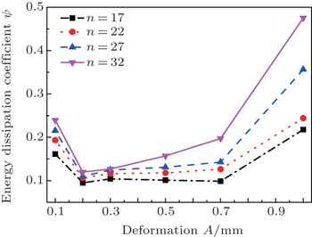
	Fig. 2. Energy dissipation coefficients versus deformation of plate damper for (a) N = 1 and δ = 0.28 mm, and (b) N = 3 and δ = 0.28 mm for different values of n.

The disadvantage of Eq. (5) is that the energy dissipation coefficient is independent of deformation amplitude, however it is possible to use this equation for calculating the average energy dissipation coefficient, besides the amplitude usually is not known before calculation. The average value of calculated energy dissipation coefficient is 0.34. The average value of energy dissipation coefficient for large deformation amplitudes of 0.1 mm,…, 1 mm (Fig. 2(a), obtained by static experiment) is 0.24. The average value of this coefficient for small deformation amplitudes of 0.01 mm, …, 0.1 mm for different values of vibration acceleration excitation a_in in a range a_in = 0.5 g, …, 2 g (obtained in dynamic experiment by vibration transfer ratio on resonance η₀ = a_out/a_in ≈ 2π/ψ, where a_out is the amplitude of acceleration on a protected object on resonance, Figs. 6(a) and 6(b)) is 0.42. Thus it is possible to use Eq. (5) for approximate engineering calculation.

For N = 3, the average value of energy dissipation coefficient for large deformation amplitudes in Fig. 2(b) is 0.14, for small deformation amplitudes in Figs. 6(c) and 6(d) it is 0.4. Average value is about 0.27. Calculation from Eq. (5) gives the result that is considerably large. The difference between two dampers is the value of φ₁, for N = 3 it is considerably large (0.858 rad). It means that for a large value of φ the value of relative displacements of layers is less than A sin φ and equation (5) needs a correction coefficient G. From experimental results, we have

For φ < 0.2, equation (6) gives G > 1. It is possible to explain why it is, by energy dissipation, not only from macro-displacement of damper deformation, but also from micro-displacements. If the damper has no waves (N = 0 and φ = 0), it also has energy dissipation coefficient (Fig. 3).

Fig. 3.

	Figure Option ViewDownloadNew Window
	Fig. 3. Energy dissipation coefficients versus deformation of plate damper without waves.

Its average value in the studied range is 0.17. Thus for φ > 0.2 it is possible to use Eq. (5) combined with correction coefficient equation (6) as follows:

For φ < 0.2 it is possible to estimate 0.17 < ψ < 0.34, and this question needs future research.

The calculated value of ψ allows the calculation of dynamic characteristics of the plate damper. For example, it is possible to use software ANSYS and harmonic analysis in this software. It is necessary to insert the value of ψ/(4π) as a coefficient of frequency independent damping DMPR. An example of this calculation is presented in Fig. 4. Results of these calculations are consistent satisfactorily with experimental results presented in Figs. 6 and 7.

Fig. 4.

	Figure Option ViewDownloadNew Window
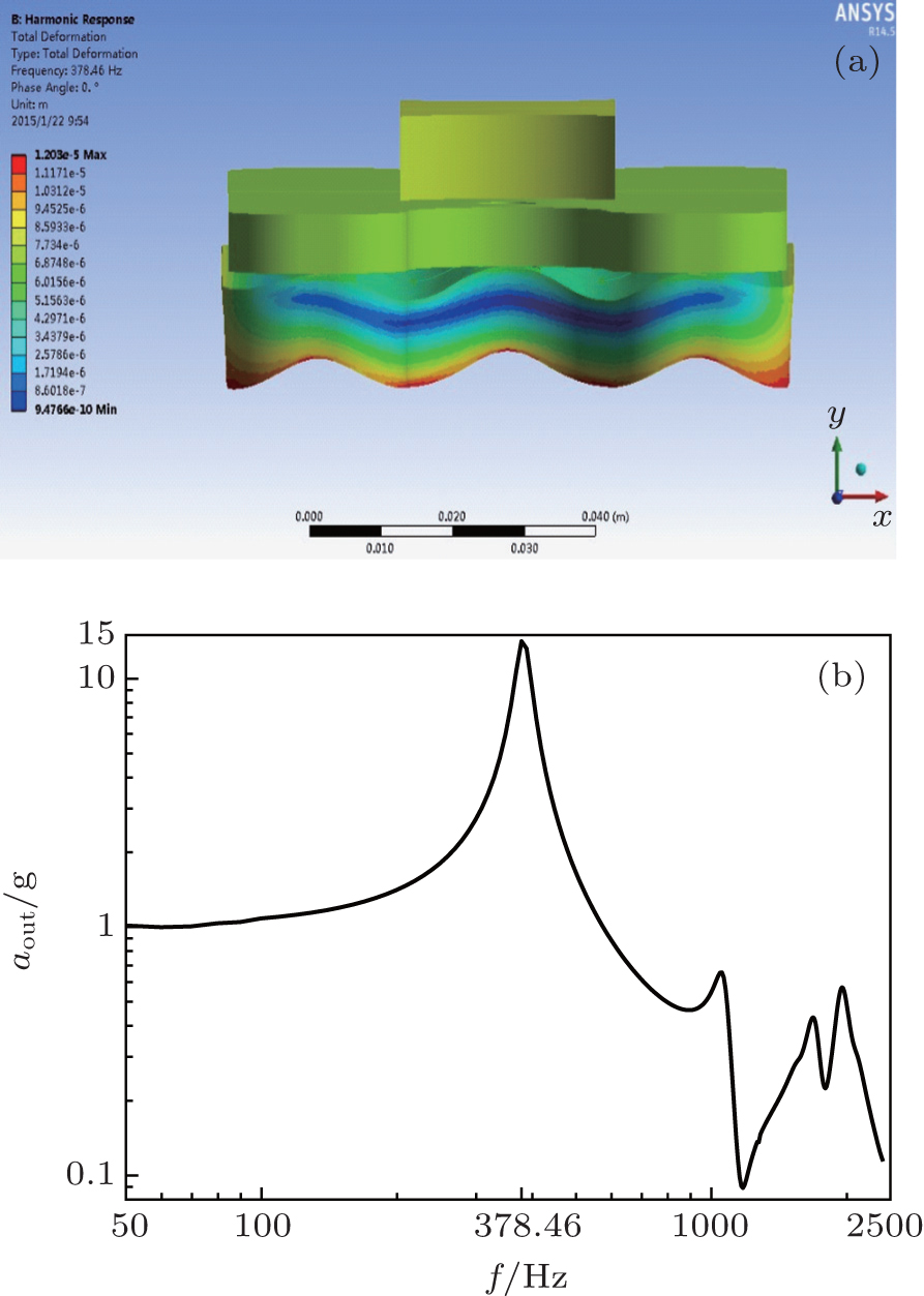	Fig. 4. Harmonic analysis of the damper by ANSYS software, showing (a) model of the damper (N = 3 and δ = 0.28 mm) and (b) amplitude–frequency characteristics.

Another way of calculating the plate damper is approximation of experimental results. By using this method, we obtain not only the harmonic vibration, but also the random load. For harmonic vibration, the own frequency f₀ and vibration transfer ratio on resonance η₀ are obtained. Some experimental results are presented in Figs. 5 and 6.

Fig. 5.

	Figure Option ViewDownloadNew Window
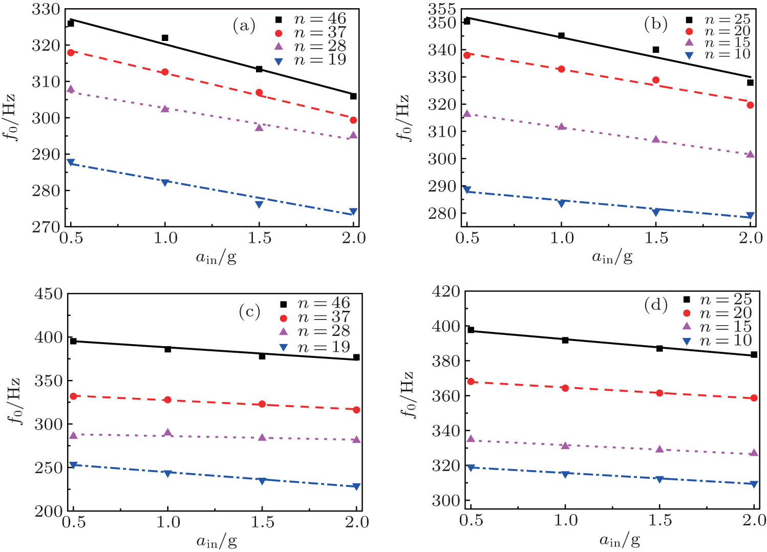	Fig. 5. Dependences of f0 on ain and n for (a) δ = 0.28 mm and N = 1, (b) δ = 0.52 mm and N = 1, (c) δ = 0.28 mm and N = 3, and (d) δ = 0.52 mm and N = 3.

Fig. 6.

	Figure Option ViewDownloadNew Window
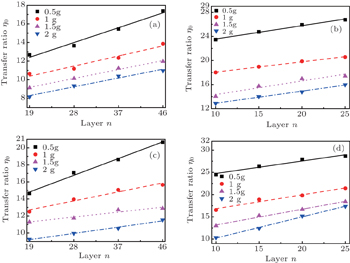
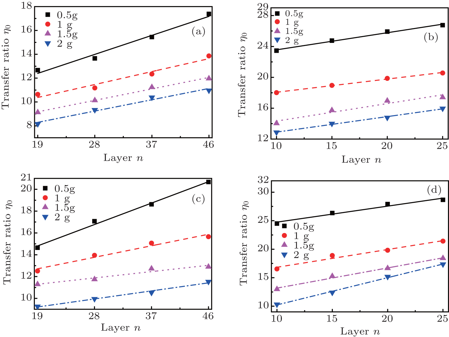	Fig. 6. Dependences of η0 on ain and n for (a) δ = 0.28 mm and N = 1, (b) δ = 0.52 mm and N = 1, (c) δ = 0.28 mm and N = 3, and (d) δ = 0.52 mm and N = 3.

For calculating the characteristics of the damper, the experimental results are approximated by linear functions. As regards frequency:

for δ = 0.28 mm and N = 1: f₀ = (265.21 + 1.55n) − (4.95 + 0.186n)a Hz (error is to 2.3%);

for δ = 0.52 mm and N = 1: f₀ = (249.42 + 4.54n) − (1.32 + 0.53n)a Hz (error is to 2.0%);

for δ = 0.28 mm and N = 3: f₀ = (152.9 + 5.2n) − (11.59 − 0.009n)a Hz (error is to 3.0%);

for δ = 0.52 mm and N = 3: f₀ = (262.1 + 5.47n) − (3.087 + 0.21n)a Hz (error is to 2.1%).

As regards vibration transfer ratio on resonance:

for δ = 0.28 mm and N = 1: η₀ = (9.94 − 1.838a) + (0.18 − 0.046a)n (error is to 7.1%);

for δ = 0.52 mm and N = 1: η₀ = (24.075 − 7.128a) + (0.205 − 0.0006a)n (error is to 9.8%);

for δ = 0.28 mm and N = 3: η₀ = (12.075 − 1.89a) + (0.235 − 0.092a)n (error is to 7.8%);

for δ = 0.52 mm and N = 3: η₀ = (26.075 − 10.71a) + (0.195 + 0.128a)n (error is to 12.4%).

For random load with different values of load power spectral density w = 0.01 g²/Hz, …, 0.03 g²/Hz, the value of root mean square acceleration is equal to the square root of the total area below the power spectral density curves, transfer ratio η_r = s₂/s₁, where s₁ is the input root mean square acceleration, s₂ is the root mean square acceleration on the protected object on resonance, and frequency of maximal output spectral density f_r are obtained. Some experimental results are presented in Figs. 7 and 8.

Fig. 7.

	Figure Option ViewDownloadNew Window
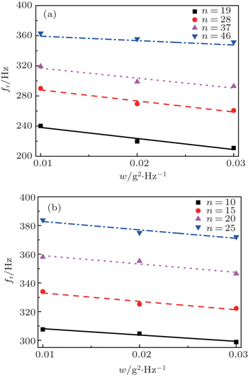
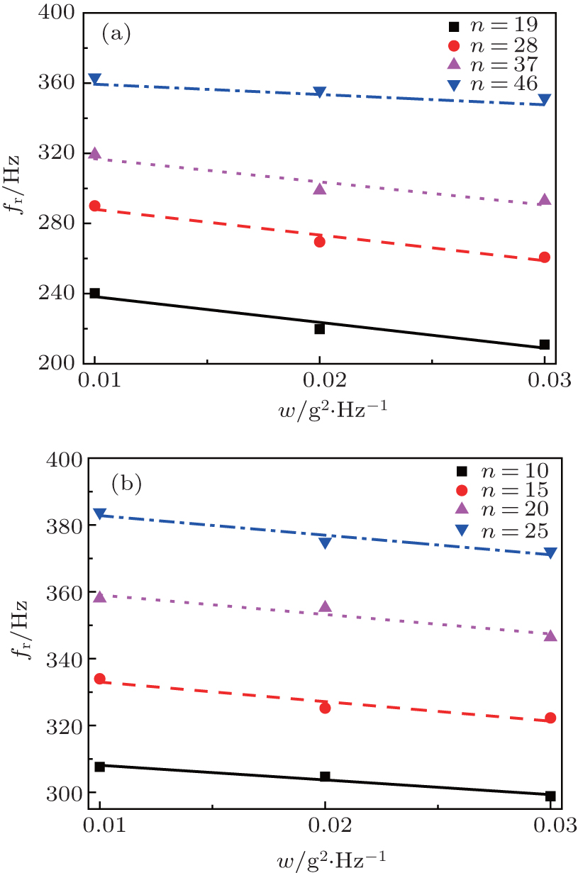	Fig. 7. Dependences of fr on w and n for (a) δ = 0.28 mm and N = 3, and (b) δ = 0.52 mm and N = 3.

Fig. 8.

	Figure Option ViewDownloadNew Window
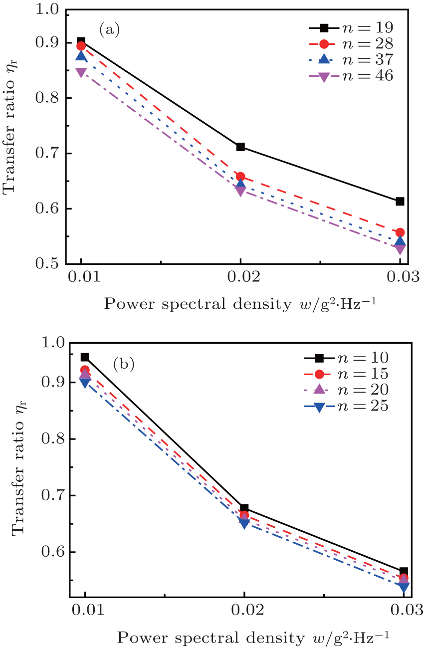	Fig. 8. Dependences of ηr on w and n for (a) δ = 0.28 mm and N = 3, and (b) δ = 0.52 mm and N = 3.

Approximation functions for frequency are as follows.

For δ = 0.28 mm and N = 3: f_r = (181.2 + 4.05n) − (2213 − 30.9n)w (error is to 3.0%);

for δ = 0.52 mm and N = 3: f_r = (262.145 + 5.09n) − (395.67 + 8.72n)w (error is to 0.9%).

Approximation functions for transfer ratio are as follows.

For δ = 0.28 mm and N = 3: η_r = (499 + 2.57n)w² − (34.4 + 0.15n)w + (1.23 − 0.0007n) (error is to 3.0%);

for δ = 0.52 mm and N = 3: η_r = (829 − 5.55n)w² − (52.5 −0.27n)w + (1.41 −0.0048n) (error is to 0.74%).

It is possible to draw some conclusions from the comparison of experimental results. Own frequency of the studied plate damper depends on total thickness of the damper, but not on the number or thickness values of the layers (for example, dampers with the same values of total thickness nδ = 46 × 0.28 = 12.88 mm and nδ = 25 × 0.52 = 13 mm have similar own frequencies seen from Fig. 5. It means that most of the layers in the damper slip in contact with other layers (in the opposite case the own frequency should increase significantly when the thickness of each layer increases, however it does not take place in experiment).

The own frequency is little dependent on input acceleration a_in: if a_in increases 4 times (from 0.5 g to 2 g), maximal changing of f₀ is 5%, usually it is less (it is the same as that for damper with N = 3). Frequency f_r is also little dependent on load power spectral density: if w increases 3 times from 0.01 g²/Hz, …, 0.03 g²/Hz, the maximal change of f_r is 10%. It is a useful property to allow an application of studied plate damper in wide ranges of vibration and random load.

Vibration transfer ratio on resonance increases if the number of layers increases, because η₀ ≈ 2π/ψ, and energy dissipation coefficient ψ increases when friction in the system increases, and it decreases when stiffness of system increases. Thus it means that if the number of layers increases, the stiffness of the studied damper increases more than friction, though the friction surface increases in this case. Therefore for a small vibration transfer ratio on resonance it is better to use the small number of layers. If the thickness value of each layer is bigger, the dependence of η₀ on n is significantly weak (Fig. 6).

Plate damper is a dry friction system. For a dry friction system if deformation amplitude is equal to zero, there is no slip in the system and ψ = 0. For non-zero deformation amplitude the value of ψ increases to any maximum and then decreases. This maximum usually lies in a range of little amplitude.

Because the studied damper has a high own frequency, its deformation amplitude on resonance is small. The whole range of vibration amplitudes obtained in dynamic experiment (from 0.01 mm to 0.1 mm) is before the maximum of ψ. Thus if input acceleration increases, the value of ψ increases too, and acceleration of the protected object increases not so much. If the input acceleration increases 4 times (from 0.5 g to 2 g), the transfer ratio on resonance significantly decreases (because η₀ ≈ 2π/ψ, Fig. 6) and acceleration on the protected object on resonance increases a little bit (more than twice) only. It is another factor for the studied damper to work stably under different levels of load.