A quantum walk in phase space with resonator-assisted double quantum dots
Bian Zhi-Hao, Qin Hao, Zhan Xiang, Li Jian, Xue Peng†,
Department of Physics, Southeast University, Nanjing 211189, China


† Corresponding author. E-mail: gnep.eux@gmail.com

Project supported by the National Natural Science Foundation of China (Grant No. 11474049) and CAST Innovation Fund.

Abstract
Abstract

We implement a quantum walk in phase space with a new mechanism based on the superconducting resonator-assisted double quantum dots. By analyzing the hybrid system, we obtain the necessary factors implementing a quantum walk in phase space: the walker, coin, coin flipping and conditional phase shift. The coin flipping is implemented by adding a driving field to the resonator. The interaction between the quantum dots and resonator is used to implement conditional phase shift. Furthermore, we show that with different driving fields the quantum walk in phase space exhibits a ballistic behavior over 25 steps and numerically analyze the factors influencing the spreading of the walker in phase space.

1. Introduction

Quantum walk (QW)[1] is appealing as an intuitive model in quantum algorithms[24] and quantum simulations,[58] because it exponentially speeds up the hitting time in glued tree graphs. Furthermore, QW offers a quadratic gain over classical algorithms on account of the diffusion spread (standard deviation), which is proportional to elapsed time t, rather than for the classical random walk (RW).[912] Thus, the conception of physical implementation of QW has become important and attracts more and more attention. Although QWs have been realized experimentally in different systems such as trapped ions,[1315] photons,[1628] nuclear magnetic resonance,[29,30] etc., the solid state system is attractive because of its stability and expected scalability.

Recently, quantum computing with quantum dots has made huge progress,[3138,4042] and the technique for coupling electrons associated with a semiconductor double-dot molecule to a microwave stripline resonator has become more and more matured. Here we make use of this technology and propose the implementation of a one-dimensional QW in phase space (PS) with superconducting resonator-assisted quantum double-dot. The walker is presented by a coplanar transmission line resonator with a single mode, and a two-level system — one electron shared by double dots via tunneling serves as the quantum coin.

In our scheme the QW is executed with indirect flipping of the coin via directly driving the resonator and allows controllable decoherence over circles in PS for observing the transition between QW and RW.[11,39,43] In the next section, we give a brief introduction of the QW in PS. In Section 3, we implement QW via realizing the walker, coin, coin flipping and conditional phase shift. In addition to the numerical analysis under the different driving fields, we observe the ballistic behavior of QW in PS and the QW–RW transmission with the influence of decoherence introduced by the shift operation in the position space.

2. Brief introduction of QW in PS

Like for the QW on a line in position space in which the walker moves towards the left or right based on the coin state, for QW on a circle in PS, the walker rotates either clockwise or counter-clockwise along the circle in PS by the same amount, say an angle Δθ, with the strictly random choice of ±Δθ through the impulse, which is applied by a harmonic oscillator.

In an ideal QW on a circle, the coin is replaced by a two-level system with internal states |0〉 and |1〉. Here we introduce the finite-dimensional orthogonal phase state representation[44]

where |n〉 is the Fock state. If the step size Δθ = 2π/d, dN, then the walker always remains on the circle with angular lattice spacing Δθ. The walker walks in PS with a state |θk〉 which can be decomposed into the phase states. Introduce the rotation operator m = eim, mZ, and we will have m|θk〉 = |θk+m〉. We choose the Hadamard operator

as the coin flipping operator and the unitary operation of one step of the QW in PS is given by

with the number operator on the walker state n = aa, a and a are the creation and annihilation operators, respectively, and is one of the Pauli operators on the coin.

We define the initial state of walker+coin system as

where |φ0〉 is the initial coin state. After N steps, the system evolves into

The walker’s phase distribution on a circle is

with d being equally spaced values of θ = θk and ρw = Trc|ϕN〉〈ϕN| is the reduced density matrix of the walker after tracing out the coin.

The standard deviation of the phase distribution, σ, which is the symbol of the spreading of the QW, is linear with respect to time t. Therefore, in sufficiently short time, the relation of phase spreading with time on a circle is a power law and satisfies[11]

where ζ is the slope coefficient and ξ is the intercept: ζ = 1 for the QW and ζ = 1/2 for the RW.

3. Physical implementation of QW
3.1. Quantum coin and walker

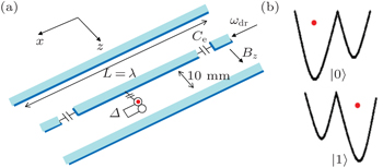
Circuit quantum electrodynamics (QED) is a device which is used to study the interaction between the quantum particle and the quantized electromagnetic mode inside a resonator. In this paper we consider a hybrid QED system of superconducting resonator-assisted quantum double-dot shown in Fig. 1(a). One of the dots, an electron that is shared by two adjacent dots coupled via tunneling, is capacitively coupled to the resonator. The double dots can be modeled as a double-well potential shown in Fig. 1(b). Generally, we apply an external magnetic field Bz of 100 mT along the axis z to the double dots.[45] Owing to the external magnetic field, there exists an energy difference between the two potentials and the electron can tunnel between the two quantum dots. We define the basis of qubits |0〉 for the electron appearing in the left dot and |1〉 for the electron in the right dot. From Fig. 1(b) we see the energy difference, namely the amount of energy consumption for moving the electron from the right dot to the left, between the states |0〉 and |1〉 is Δ = T, where T is the rate of electron tunneling in the different dots.

Fig. 1. (a) Experimental proposal for QW with superconducting resonator-assisted quantum double-dot. The red dot represents the electron. The coupling between the resonator and the double-dot can be switched on and off via an external electric field along the x axis. The superducting resonator is driven by a field along the x axis for implementing the coin flipping. (b) The double-dot modeled as a double-well potential. The basis of the qubit states represents the electron either in the left or right potential via tunneling. The energy difference between the states |0〉 and |1〉 is Δ.

After applying the magnetic field to the quantum dots, the double-well potential forms a circuit.[46] We just consider one circumstance, i.e., whether the electron is located in the left dot or right, the Hamiltonian describing the circuit is given by

where Ec = e2/2Ctot is the charge energy, Ctot = Cg + CJ is the total capacitance in the circuit, CJ is the Josephson capacitance and Cg is voltage biased from a lead having capacitance to the circuit, Ng = CgVg/2e is the gate charge which represents the total polarization charge. Restricting the gate charge to the range Ng ∈ [0,1] by using the voltage Vg, the Hamiltonian in Eq. (8) is rewritten as

So far, we have shown the Hamiltonian of the double-well potential. From Eq. (9) we see that the double-well potential presents the double-dot system with effective electric fields along the x and z directions, and the system with internal states |0〉 and |1〉 can be used as a two-level quantum coin.

Now we consider the circuit QED of double dots coupled to a superconducting resonator. The dots are located in the center of the resonator. If the oscillator mode of the resonator is coupled to the double-dot, by using the coordinate system transformation

and choosing 2Ng = 1, θ = π/2, the Hamiltonian of the interacting qubit and resonator system with the rotating wave approximation takes the form (ħ = 1)

where ωc is the frequency of the resonator, and Ω[47] is the resonator-induced energy splitting of the qubit:

and

is the vacuum Rabi frequency. The form of Hamiltonian in Eq. (10) is the well-known Jaynes–Cummings (JC) model.[48]

3.2. Coin flipping and conditional phase shift operator

In our hybrid system, the walker can be represented by the phase state of the single mode of the resonator and the coin is the two-level energy system. To implement the coin flipping operator, a microwave time-dependent driving field is applied to the circuit QED system with the form

where ωd is the frequency of driving field. Let ɛ(t) be a square wave, so ɛ is a constant when the field is turned on, while if it is zero, then the field is off. The Hamiltonian of the hybrid system, containing the driving field, is

In the dispersive regime,

To calculate the effective Hamiltonian from Eq. (12), we introduce the unitary transformation = exp[g/δ(aσ+aσ)], and use the translation equation tot,[46,49] the Hamiltonian in Eq. (12) turns into the effective Hamiltonian of the whole system with driving field

with , , , and .

The free evolution

continues even when the driving field is off (ɛ = 0).

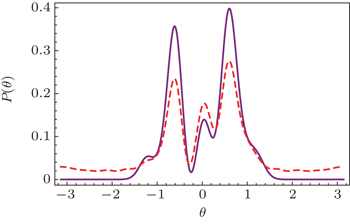
By choosing the coherent state |α = 3〉 and different values of ɛ, we show the probability distribution of the walker in PS at the 4th step with step size Δθ = 0.3 (Fig. 2). The solid line represents the circumstance with ɛ = 0.01 GHz, whereas the dashed line represents the circumstance with ɛ = 0.012 GHz. From Fig. 2 we see that the peak probability with ɛ = 0.012 GHz is smaller than that with ɛ = 0.01 GHz because the evolution of the last term in Eq. (14) provides a displacement operator in position space and pushes the walker off the circle in PS. Apart from this, the rate of probability on the position θ = 0.01 GHz in the three main peaks with ɛ = 0.012 GHz is higher than that with ɛ = 0.01 GHz, that is to say, the decoherence drives the probability to the origin position, making the distribution be Gaussian distribution. These can be regarded as the decoherence on the walker in PS and with decoherence increasing we can observe the QW–RW transmission.

Fig. 2. The probability distributions of the walker in PS at the 4th step with the initial walker state |α = 3〉 and coin state , the step size Δθ = 0.3, and ɛ = 0.01 GHz in solid line and ɛ = 0.012 GHz in dashed line respectively. The phase distribution shows a ballistic behavior of the QW in PS. With the strength of the driving field increasing, the decoherence introduced by displacement in position space increases and the phase distribution tends to be the combination of those of QW and RW.

The evolution of the hybrid system is described by the effective Hamiltonian. The first term on the right-hand side in Eq. (14) contains aaσz, which proves an interrelated relationship between the walker and coin, and makes the walker evolve along clockwise or counterclockwise at the same constant angle with the orientation based on the state of the coin. The second and third terms involve the operators σz and aa, which represent the consequent frequency of walker and the energies for the coin, respectively. The fourth term contains σx and it can translate into the Hadamard coin flip by choosing a suitable pulse time. The coefficient is proportional to the Rabi frequency. The last term is the displacement in the position space and pushes the walker off the circle in PS. Thus it also causes the decoherence in the QW in PS.

4. Numerical analysis

Now all the factors that the implementation of QW needs are fulfilled. To make the scheme work, the value of constant coefficient ɛ in the last term in Eq. (14) which brings the displacement in PS must be kept very small. Nevertheless, the Rabi frequency Ω2 is proportional to the pulsed driving field ɛ, so, no matter how small the value of ɛ is, we can choose a suitable pulse time to transform the σx into Hadamard coin flip.

We choose the initial coin state as

set the initial field in the resonator as coherent state

and obtain the realistic system parameters as follows:[50,51]

In Fig. 3(a), we show the ln–ln plots of the standard deviation of the probability distribution of the walker in PS with step size Δθ = 0.3 only even steps without losing generality, the diamonds, squares, stars, triangles represent the standard deviations of the phase distribution of QW in PS with different ɛ = (0.01,0.012,0.015,0.018) GHz, respectively. With the step number increasing, the wave function of the walker meets itself on the circle in PS after 15 steps. Thus after 15 steps, the curve of the ln–ln plot of standard deviation versus the step number drops down. This shows the difference from the QW on the line, though for the first few steps QWs on both circle and line show the ballistic behavior as expected. Overall, the slope of the points becomes small with increasing constant ɛ. To realize the scenario more intuitively, we cut out the standard deviation after 6, 8, and 10 steps and connect the points into a line of the whole circumstance (Fig. 3(b)). The figure shows the slopes of the line ς which correspond to the diamonds, squares, stars, triangles are about 1, 0.89, 0.64, 0.53 respectively. Using Eq. (7) as a reference, the slopes are 1 for QW and 0.5 for RW respectively, different slopes of the ln–ln plots show the different behaviors of the walker on the circle in PS with different levels of decoherence. The decoherence is introduced by the driving field which leads the walker to move in position space too. For QW in PS, it is equivalent to decoherence. With the strength of the driving field increasing the decoherence increases. Hence with decoherence increasing we see the QW–RW transition. With increasing the value of ɛ, the trend QW changes to RW is more obvious. So, in order to keep the more prominent properties of QW, ɛ must be small enough.

Fig. 3. (a) The ln–ln plots of the standard deviation of the phase distribution σ versus step number N with the initial walker state |α = 3〉, coin state and different field strengths with ɛ = (0.01,0.012,0.015,0.018) GHz, the step size in PS Δθ = 0.3. The dots represent the standard deviation of even steps up to 25 steps. (b) The ln–ln plots with various ɛ values showing the slopes of the plots which represent the values of the walker spreading speed ς.
5. Conclusions

We show how a QW in PS can be implemented in a quantum quincunx created through superconducting resonator-assisted quantum double dots and how interpolation from a quantum to a random walk is implemented by controllable decoherence introduced by the displacement of the walker in position space. Our scheme shows how a QW with just one walker can be implemented in a realistic system. The coin flipping operation is implemented by driving the resonator directly, and at the same time the driving field also introduces the displacement of the walker in position space and pushes the walker off the circle in PS. Thus the displacement in position space is equivalent to decoherence on the walker in PS which is controlled by the strength of the driving field. With the strength of the driving field increasing the decoherence increases and we observe the QW–RW transition.

Although in our paper we make use of the decoherence introduced by the driving field to show the transition from QW to RW, which is one of the main points of our paper, for most of the applications of QW it requires quadratic enhancement of walker spreading. The decoherence induced by the driving field can be compensated for by the method in Ref. [11]. The displacement of the walker in position space pushes the walker off the circle in PS by changing the mean photon number of the resonator field. Hence we can adjust the pulse duration each time ti according to the predicted mean photon number (i), that is, ti = [δ + 2(i)−2gɛ/δ]π/4gɛ, to compensate for the effect due to the displacement and obtain a perfect QW in PS.

Reference
1Aharonov YDavidovich LZagury N 1993 Phys. Rev. A 48 1687
2Ambainis A 2003 Int. J. Quantum Inform. 1 507
3Childs A MCleve RDeotto EFarhi EGutmann SSpielman D A2003Proc. 35th ACM Symposium on Theory of Computing (STOC 2003)5968
4Shenvi NKempe JWhaley K B 2003 Phys. Rev. A 67 052307
5Zhang RXu YXue P 2015 Chin. Phys. B 24 010303
6Zhang RXue PTwamley J 2014 Phys. Rev. A 89 042317
7Zhang RXue P 2014 Quantum Information Processing 13 1825
8Zhang RQin HTang BXue P 2013 Chin. Phys. B 22 110312
9Brun T ACarteret H AAmbainis A 2003 Phys. Rev. Lett. 91 130602
10Xue PSanders B C 2008 New J. Phys. 8 053025
11Xue PSanders B CBlais ALalumiére K 2008 Phys. Rev. A 78 042334
12Hardal A CXue PShikano YMüstecaploǧlu Ö ESanders B C 2013 Phys. Rev. A 88 022303
13Zähringer FKirchmair GGerritsma RSolano EBlatt RRoos C F 2010 Phys. Rev. Lett. 104 100503
14Schmitz HMatjeschk RSchneider ChGlueckert JEnderlein MHuber TSchaetz T 2009 Phys. Rev. Lett. 103 090504
15Xue PSanders B CLeibfreid D 2009 Phys. Rev. Lett. 103 183602
16Bouwmeester DMarzoli IKarman G PSchleich WWoerdman J P 1999 Phys. Rev. A 61 013410
17Do BStohler M LBalasubramanian SElliott D SEash CFischbach EFischbach M AMills AZwickl B 2005 J. Opt. Soc. Am. B 22 499
18Zhang PRen X FZou X BLiu B HHuang Y FGuo G C 2007 Phys. Rev. A 75 052310
19Peruzzo ALobino MMatthews J C FMatsuda NPoliti APoulios KZhou XLahini YIsmail NWÖrhoff KBromberg YSilberberg YThompson M GO’Brien J L 2010 Science 329 1500
20Perets H BLahini YPozzi FSorel MMorandotti RSilberberg Y 2008 Phys. Rev. Lett. 100 170506
21Sansoni LSciarrino FVallone GMataloni PCrespi ARamponi ROsellame R 2012 Phys. Rev. Lett. 108 010502
22Jeong Y CDi Franco CLim H TKim M SKim Y H 2013 Nat. Commun. 4 2471
23Broome M AFedrizzi ALanyon B PKassal IAspuru-Guzik AWhite A G 2010 Phys. Rev. Lett. 104 153602
24Xue PQin HTang BSanders B C 2014 New J. Phys. 16 053009
25Schreiber ACassemiro K NPotoček VGábris AMosley P JAndersson EJex ISilberhorn C 2012 Science 336 55
26Xue PQin HTang B 2014 Sci. Rep. 4 4825
27Xue PQin HTang BZhan XBian Z HLi J 2014 Chin. Phys. B 23 110307
28Bian Z HLi JQin HZhan XZhang RSanders B CXue P 2015 Phys. Rev. Lett. 114 203602
29Chen H WKong XChong BQin GZhou X YPeng X HDu J F 2011 Phys. Rev. A 83 032314
30Kuznetsova M SFlisinski KGerlovin I YaPetrov M YuIgnatiev I VYu Verbin SYakovlev D RReuter DWieck A DBayer M 2014 Phys. Rev. B 89 125304
31Culcer DSaraiva A LKoiller BHu X DSarma S D 2012 Phys. Rev. Lett. 108 126804
32Paudel H PLeuenberger M N 2013 Phys. Rev. B 88 085316
33Petta J RJohnson A CTaylor J MLaird E AYacoby ALukin M DMarcus C MHanson M PGossard A C 2005 Science 309 2180
34Johnson A CPetta J RTaylor J MYacoby ALukin M DMarcus C MHanson M PGossard A C 2005 Nature 435 925
35Solenov DEconomou S EReinecke T L 2013 Phys. Rev. B 87 035308
36Burkard GImamoglu A 2006 Phys. Rev. B 74 041307
37Lin Z RGuo G PTu TZhu F YGuo G C 2008 Phys. Rev. Lett. 101 230501
38Golovach V NBorhani MLoss D 2010 Phys. Rev. A 81 022315
39Burda ZDuda JLuck J MWaclaw B 2009 Phys. Rev. Lett. 102 160602
40Xue P 2013 J. Comput. Theor. Nanosc. 10 1
41Tang BQin HZhang RLiu J MXue P 2014 Chin. Phys. B 23 050307
42Xue P 2010 Phys. Lett. A 374 2601
43Xue PSanders B C 2013 Phys. Rev. A 87 022334
44Sanders B CBartlett S DTregenna BKnight P L 2003 Phys. Rev. A 67 042305
45Taylor J MEngel H ADür WYacoby AMarcus C MZoller PLukin M D 2005 Nat. Phys. 1 177
46Blais AHuang R SWallra AGirvin S MSchoelkopf R J 2004 Phys. Rev. A 69 062320
47Schoelkopf RClerk AGirvin SLehnert KDevoret M2003Quantum Noise in Mesoscopic PhysicsDordrechtKluwer AcademicChap. 9, pp. 175–203
48Jaynes E TCummings F W 1963 Proc. IEEE 51 89
49James D FJerke J 2007 Can. J. Phys. 85 625
50Schuster D IHouck A ASchreier J AWallraff AGambetta J MBlais AFrunzio LMajer JJohnson BDevoret M HGirvin S MSchoelkopf R J 2007 Nature 445 515
51Blais AGambetta JWallraff ASchuster D IGirvin S MDevoret M HSchoelkopf R J 2007 Phys. Rev. A 75 032329