


Improved kernel gradient free-smoothed particle hydrodynamics and its applications to heat transfer problems
[Lei Juan-Mian†,  , Peng Xue-Ying]
, Peng Xue-Ying]
|
|


† Corresponding author. E-mail:
Kernel gradient free-smoothed particle hydrodynamics (KGF-SPH) is a modified smoothed particle hydrodynamics (SPH) method which has higher precision than the conventional SPH. However, the Laplacian in KGF-SPH is approximated by the two-pass model which increases computational cost. A new kind of discretization scheme for the Laplacian is proposed in this paper, then a method with higher precision and better stability, called Improved KGF-SPH, is developed by modifying KGF-SPH with this new Laplacian model. One-dimensional (1D) and two-dimensional (2D) heat conduction problems are used to test the precision and stability of the Improved KGF-SPH. The numerical results demonstrate that the Improved KGF-SPH is more accurate than SPH, and stabler than KGF-SPH. Natural convection in a closed square cavity at different Rayleigh numbers are modeled by the Improved KGF-SPH with shifting particle position, and the Improved KGF-SPH results are presented in comparison with those of SPH and finite volume method (FVM). The numerical results demonstrate that the Improved KGF-SPH is a more accurate method to study and model the heat transfer problems.
Grid-based numerical methods such as the finite element method (FEM) and finite difference method (FDM) have been widely applied to various fields of computational fluid dynamics (CFD) and computational solid dynamics (CSD). However, conventional grid-based methods suffer some inherent difficulties in many aspects, such as mesh generation for irregular or complex geometry and cases with heavily distorted mesh. So many meshless methods have been developed over the past twenty years, such as element-free Galerkin method,[1–3] complex variable meshless method,[4,5] finite point method,[6] reproducing kernel particle method,[7–9] smoothed particle hydrodynamics,[10,11] moving particle semi-implicit method,[12] and corrective smoothed particle method.[13]
Smoothed particle hydrodynamics (SPH)[14] is a transient, Lagrangian method, proposed by Lucy,[15] Gingold and Monaghan[16] in 1977. The SPH was originally invented for modeling the astrophysical phenomena in three-dimensional (3D) open space, and now has been widely applied to fluid dynamics such as numerical simulation of quasi-incompressible flows,[17] multi-phase flows[18] and heat conduction.[19] In the SPH, a set of particles associated with physical properties are used to represent the state of the system. Since these particles can move within the computational domain in the Lagrangian frame, SPH is an attractive tool to model complex flows with free surfaces, moving interfaces and large deformations which are difficult for grid-based methods. Though the SPH has a very wide range of applications in incompressible flows,[20–22] applications in heat transfer problems are still not mature enough.
Natural convection in a closed square cavity is a classic convection heat transfer problem, which is important not only for understanding heat transfer phenomena but also for studying problems such as cooling of electrical equipment, nuclear reactor systems and crystal growth in liquids.[23] Hence, studies of heat transfer problems and obtaining their accurate solutions are still significant. In 1998, by using the SPH, Cleary[24] modeled natural convective flows in a differentially heated square cavity for low and moderate Rayleigh numbers (102, 104, 105). The results showed that the SPH is sufficient to give excellent isotherms for low Ra, but when Ra = 105, obvious deviations appear between SPH results and FEM results. Chaniotis et al.[25] used the remeshed SPH to simulate natural convection in a differentially heated cavity, displayed the contours of temperature and vorticity for Ra = 103 and 104, and the relative error between the remeshed SPH solution and the benchmark solution of de Vahl Davis is less than 8%. Szewc et al.[26] modeled natural convection with SPH based on non-Boussinesq formulation, the local Nusselt number distributions look very realistic, but contours for temperature and velocity are not smooth. Though it has been widely used in the field of solid mechanics and fluid mechanics, the conventional SPH is still poor in stability and accuracy.
One of the factors causing SPH instability is the non-uniform particle distribution.[27] In the Lagrangian numerical simulation, particles move along the streamlines, which will cluster or scatter under certain conditions, such as natural convection. What is more, the non-physical behavior of the kernel function will weaken the interaction between particles when particle distances are within a close range. Then particles will continue to cluster, which will reduce the precision or interrupt the numerical simulation, so it is necessary to correct the particle position. In 2008, Nester et al.[28] proposed a particle velocity correction, and applied this method to the finite volume particle method (FVPM) to maintain the uniformity of the moving particle cloud. In 2009, particle velocity correction was improved by Xu et al.,[29] and the new approach called shifting particle position maintains accuracy and stability when simulating Taylor–Green vortices and vortex spin-down problems. In 2012, Hashemi et al.[30] applied shifting particle position to SPH, the numerical results demonstrate that shifting particle position can alleviate defects produced by non-uniform distribution of particles and improve the stability of the numerical method. Shifting particle position not only needs less computational time but also effectively maintains the uniformity of particle distribution. Hence, this paper uses shifting particle position to weaken the non-uniform particle distribution effects on numerical simulation.
At present, in order to overcome the low accuracy of the conventional SPH, a large number of methods have been proposed. Finite particle method (FPM)[31] is an enhanced version of SPH, in which the function and its first derivatives are calculated simultaneously to restore the particle consistency and improve the approximation accuracy. Zhang and Batra[32] used numerical tests to show the FPM superiority over the CSPM, and the simulation results of the 2D transient heat conduction problems demonstrate that FPM is more accurate than CSPM. Liu et al.[31] modeled the classic Poiseuille flow, Couette flow, shear driven cavity and a dam collapsing problem by FPM, and the numerical examples showed that the FPM is a very attractive alternative for simulating incompressible flows. On the basis of FPM, Huang et al.[33] substituted the product of particle distance and kernel function for kernel gradient in FPM since the kernel gradient is not necessary in the whole computation, and this new approach is referred to as a kernel gradient free-SPH (KGF-SPH). KGF-SPH widens the selection of the kernel function, improves the simulation precision and simplifies the solving process because of the symmetric property of the corrective matrix. However, the conventional FPM and KGF-SPH differentiate the first derivatives to obtain the second derivatives, and the errors of the first derivatives will be brought into the second derivatives, which will reduce the accuracy of the simulation results.
In the present paper, the Improved KGF-SPH is proposed, which modifies the two-pass model in KGF-SPH with a new kind of discretization scheme for the Laplacian. Simple (1D and 2D heat conduction) and complex (natural convection in a closed square cavity) heat transfer problems are simulated by the Improved KGF-SPH. The rest of this paper is organized as follows. The conventional SPH, KGF-SPH, and Improved KGF-SPH are introduced in Section 2. In Section 3, the Improved KGF-SPH formulations for the governing equations and the state equation are briefly depicted. In Section 4, the particle shifting position is presented in detail. In Section 5, the 1D and 2D heat conduction problems are adopted to test the precision and stability of the Improved KGF-SPH. In Section 6, natural convection in a closed square cavity is modeled by the Improved KGF-SPH with shifting particle position. In Section 7, some conclusions are drawn from the present research results.
The concept behind SPH is based on an interpolation scheme, and in SPH, any function or physical property can be approximated by its value at a set of disordered points. The formulations of SPH are often divided into two key steps: the first step is the integral representation or the so-called kernel approximation of physical properties, the second one is the particle approximation of physical properties. In the first key step, for an arbitrary function f, the kernel approximation of the function value f (


In the particle approximation, the computational domain is discretized by a series of particles with some attributes such as mass, position, momentum and energy. Equations (


In 2D case, the most widely used SPH discretization scheme for the Laplacian is[34]


In 2015, based on FPM, Huang et al.[33] developed a kernel gradient free-SPH (KGF-SPH) which only involves kernel function itself in kernel and particle approximation. In the KGF-SPH, performing Taylor series expansion at a certain point


In 2D space, equation (


It can be observed from Eq. (
The two-pass model, which obtains second derivatives by nesting two first derivative operations, is used to discretize the Laplacian in the conventional KGF-SPH. So in 2D space, the KGF-SPH discretization scheme for the Laplacian is


In KGF-SPH, the Laplacian is calculated by using Eq. (
In order to overcome these two drawbacks, in this paper we propose a new discretization scheme to approximate the Laplacian, and apply it to the KGF-SPH. The following section provides the derivation process of the new Laplacian discretization scheme in detail.
In 2D space, performing Taylor series expansion at a nearby point (xi, yi) and retaining the second derivatives, a function f at point (xj, yj) can be expressed as follows:

Multiplying both sides of Eq. (


Equations (
For natural convection in a closed square cavity, assuming the dynamic viscosity coefficient μ to be a constant, the governing equations in the Lagrangian frame are[14]


Using Eqs. (


The above governing equation is not closed, so the state equation should be added. In this paper, the following weakly compressible state equation is used[17]

In order to enhance numerical stability, shifting particle position can be used to maintain the uniformity of particles. Shifting particle position employed in this paper modifies the particle position, and the position shift δ


Since the particles are shifted, the physical properties carried by particles are also changed. The physical properties are corrected by the following equation:

In order to validate the Improved KGF-SPH, two simple conduction heat transfer problems are studied in this section. The Improved KGF-SPH results are compared with those from SPH, KGF-SPH, and analytical solutions to show the high accuracy and stability of the Improved KGF-SPH.
The computational domain for 1D heat conduction in this paper is the line segment from 0 to 1, at t moment, the temperature T(x, t) is governed by the following heat conduction equation:


Figure
 | Fig. 1. Particle distribution for 1D heat conduction. |
Figure
 | Fig. 2. Temperature profiles at t = 0.2 s for 1D heat conduction. |
In this section, the Improved KGF-SPH formulations are applied to the 2D heat conduction case with a simple square cavity geometry whose side length is L. At t moment, the temperature T(x,y,t) is governed by

Figure
 | Fig. 3. Schematic diagram and particle distribution for 2D heat conduction. |
In order to verify our numerical method, the solution of the 2D heat conduction problem by the finite particle method (FVM) with 101×101 nodes is taken as a reference solution. For the SPH, KGF-SPH, and Improved KGF-SPH, 11×11 and 21×21 uniformly distributed particles are employed.
Figure
 | Fig. 4. Temperature distribution along the line x = 0.05 m for 2D heat conduction. (a) 11×11 particles, (b) 21×21 particles. |
In order to show the Improved KGF-SPH superiority over SPH and KGF-SPH clearly, figure
 | Fig. 5. Temperature variations with time for monitor particle A. |
The Improved KGF-SPH with shifting particle positions is used to model natural convections in a closed square cavity at different Rayleigh numbers in this section. In order to verify our Improved KGF-SPH formulation, the Improved KGF-SPH results are compared with the corresponding SPH and FVM simulation results.
Schematic diagram for natural convection in a closed square cavity is provided in Fig.
 | Fig. 6. Schematic diagram for natural convection in a closed square cavity. |
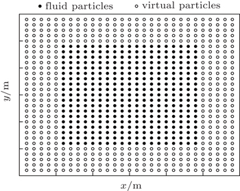
Particle distribution for natural convection in a closed square cavity is shown in Fig.
 | Fig. 7. Particle distribution for natural convection in a closed square cavity. |
Natural convection in a closed square cavity is studied at Ra = 104, 105 and 106 to validate the Improved KGF-SPH. In this case, the Prandtl number Pr = μ/(ρ α) = 0.71, the dynamic viscosity coefficient μ = 1.707 × 10⁻⁵ kg/m·s, density ρ = 1.225 kg/m3, the thermal diffusion coefficient α = 1.963× 10⁻⁵ m2/s, the thermal expansion coefficient βT = 4.095 × 10⁻³ K−1. TH = 283 K, TC = 273 K, and the initial temperature of the fluid inside the square cavity is T0. The reference density ρ∞ in state equation is set to be 1.225 kg/m3, and for convenience, the artificial sound speed c values are set to be 0.25 m/s, 0.4 m/s and 0.8 m/s for Ra = 104, 105, and 106 respectively. In this paper, the size of Rayleigh number Ra is adjusted by changing the sizes of g and L. In the numerical simulation of natural convection in a closed square cavity, shifting particle position is adopted to improve the numerical stability.
There are two kinds of boundary conditions in natural convection problems: adiabatic boundaries and isothermal boundaries. In this paper, we use the projecting method proposed by Huang et al.[33] to calculate physical properties of virtual particles. The projecting method first finds out the normal direction
 | Fig. 8. Boundary treatment. |
The adiabatic boundary condition is a Neumann-type boundary condition with ∂T/∂


The isothermal boundary condition is a Dirichlet-type boundary condition. On the isothermal boundaries, the position vectors of virtual particles and projecting points satisfy the following relations:


For natural convection in a closed square cavity with Ra = 104, g = 8.350 m/s2, L = 0.02 m, 149×149 fluid particles are evenly placed in the computational domain. Figures
 | Fig. 9. Temperature T contours for Ra = 104 obtained by different methods: (a) FVM, (b) SPH, and (c) Improved KGF-SPH. |
 | Fig. 10. Horizontal velocity u contours for Ra = 104, obtained by different methods: (a) FVM, (b) SPH, and (c) Improved KGF-SPH. |
 | Fig. 11. Vertical velocity v contours for Ra = 104, obtained by different methods: (a) FVM, (b) SPH, and (c) Improved KGF-SPH. |
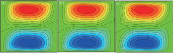
The simulations for Ra = 105 are performed with 149×149 fluid particles, g = 5.344 m/s2, L = 0.05 m, and the temperature contours t t = 20 s are presented in Fig.
 | Fig. 12. Temperature T contours for Ra = 105 obtained by different methods: (a) FVM, (b) SPH, and (c) Improved KGF-SPH. |
 | Fig. 13. Horizontal velocity u contours for Ra = 105 obtained by different methods: (a) FVM, (b) SPH, and (c) Improved KGF-SPH. |
 | Fig. 14. Vertical velocity v contours for Ra = 105 obtained by different methods: (a) FVM, (b) SPH, and (c) Improved KGF-SPH. |
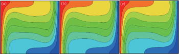
For Ra = 106, g = 6.680 m/s2, L = 0.1 m, the boundary layer becomes thinner with Rayleigh number increasing, so more particles (199×199 fluid particles) are used to model the natural convection in a closed square cavity. Figure
 | Fig. 15. Temperature T contours for Ra = 106 obtained by different methods: (a) FVM, (b) SPH, and (c) Improved KGF-SPH. |
 | Fig. 16. Horizontal velocity u contours for Ra = 106 obtained by different methods: (a) FVM, (b) SPH, and (c) Improved KGF-SPH. |
 | Fig. 17. Vertical velocity v contours for Ra = 106 obtained by different methods: (a) FVM, (b) SPH, and (c) Improved KGF-SPH. |
There are two distinct flow patterns for natural convection in a closed square cavity: heat conduction and heat convection. It can be seen from Figs.
It can be seen from Fig.
In order to validate the accuracy of Improved KGF-SPH, the velocity profiles obtained by SPH and Improved KGF-SPH are compared with those of FVM. For convenience, the dimensional variables are non-dimensionalized by the following equations: x* = x/L, y* = y/L, u* = uL/α, v* = vL/α. The non-dimensional horizontal velocity u* distribution along the mid-width (x = L/2) and non-dimensional vertical velocity v* along mid-height (y = L/2) over the Ra range of 104 to 106 are presented in Figs.
 | Fig. 18. Non-dimensional velocity profiles along central lines: (a) non-dimensional horizontal velocity u*, and (b) non-dimensional vertical velocity v*. |
The maximum non-dimensional horizontal velocity 


| Table 1. Comparison of maximum non-dimensional velocity at central lines. . |
A new Laplacian discretization scheme is proposed to avoid bringing errors of the first derivatives to the second derivatives in the KGF-SPH kernel and particle approximation. The superiority of the new Laplacian discretization scheme applied in KGF-SPH is verified by modeling 1D and 2D heat conduction problems. The Improved KGF-SPH is successfully used to study natural convection in a closed square cavity with Ra = 104, 105, and 106. It can be seen that the SPH overestimates the heat transfer, the KGF-SPH results oscillate violently, while the Improved KGF-SPH results accord well with the analytical solution and the reference solution. The Improved KGF-SPH is more accurate than SPH and stabler than KGF-SPH, thus it is an attractive tool to study and model the heat transfer problems. In this paper, only 1D and 2D simulations are done; as a next step, our method can be extended to solving 3D heat transfer problems. Furthermore, the application of the proposed method can be broadened to other problems controlled by governing equations, such as viscous fluid flow.
| 1 | |
| 2 | |
| 3 | |
| 4 | |
| 5 | |
| 6 | |
| 7 | |
| 8 | |
| 9 | |
| 10 | |
| 11 | |
| 12 | |
| 13 | |
| 14 | |
| 15 | |
| 16 | |
| 17 | |
| 18 | |
| 19 | |
| 20 | |
| 21 | |
| 22 | |
| 23 | |
| 24 | |
| 25 | |
| 26 | |
| 27 | |
| 28 | |
| 29 | |
| 30 | |
| 31 | |
| 32 | |
| 33 | |
| 34 | |
| 35 | |
| 36 |