Electric double layer exists widely in biology and materials. Nowadays, the demand on the higher energy density of the supercapacitor has become stronger, due to its high power density. Graphene with a high surface area as well as the ionic liquid (IL) with many unique properties, make them highly desirable. Thus, a theoretical understanding on the capacitance behavior on such newly developed materials is greatly needed. Over the past 100 years, a mean-field theory (MFT), such as the Gouy–Chapman EDL model, is referred to frequently. Later, the re-discovery and new development of the mean field based EDL theory also attracted a great deal of attention. In this review, we briefly overview the development of mean field based EDL theory.

The first EDL model was proposed by Helmholtz, ^{[ 1 , 2 ]}

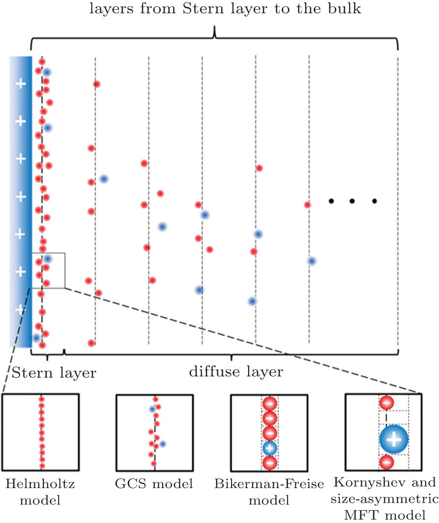
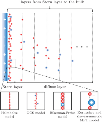
Equation ( 1 ) provides a vivid picture for the electrochemical capacitor or the so-called supercapacitor. Considering the interface between a charged electrode and ionic electrolyte, as depicted in Fig. 1 , the counterions will accumulate on the electrode due to the electrostatic interactions. Such arrangement may be analogous to the parallel plate capacitor, with the other plate forming by the counter ion layer. A distinct feature of such a capacitor is that the distance between the two “plates” is much shortened. Theoretically, the distance is often attributed to the radius of the ions on the nanometer scale. Due to such short distance d , the capacitance C _H by Eq. ( 1 ) is much enhanced, and a capacitor formed by such EDL is the so-called electrochemical capacitor or supercapacitor.

Fig. 1.

	Figure Option View Download New Window
	Fig. 1. Scheme of electric double layer (EDL). The single charged ion layer adjacent to the electrode forms the compact layer or Stern layer, while the outer layer forms the diffuse layer. The series of the two layers is called the Gouy–Chapman–Stern (GCS) EDL model.

Since such a simple and clear picture is given by Eq. ( 1 ), it is frequently adopted experimentally for the supercapacitance behavior. ^{[ 3 ]} It is also notable that Eq. ( 1 ) is a highly simplified model, nevertheless in a real electrolyte solution, the EDL structure is much more complicated. Clearly, the distribution of the counterions is not a single charged layer close to the electrode surface. A more realistic picture is the diffuse layer as in Fig. 1 , as proposed by Gouy ^{[ 4 ]} and Chapman. ^{[ 5 ]}

In the Gouy–Chapman model, the number density of monovalence ion in the electrolyte solution is given by the Boltzmann distribution

Equation ( 3 ) gives charge density of 1:1 electrolyte system, for which an analytical expression of differential capacitance is available. Appling Poisson equation, i.e.,

This Gouy–Chapman model in Eq. ( 5 ) differs from the Helmholtz model of Eq. ( 1 ) in its extra dependence on ϕ ₀ . From the electrochemical perspective, C _d in Eq. ( 5 ) is the natural response of the electrode potential dependent EDL at different ϕ ₀ , which alters EDL structures and results in different C _d . However, the hyperbolic cosine function in Eq. ( 5 ) implies that C _d increases with ϕ ₀ , and this never happens in reality. In order to remedy this, Stern ^{[ 6 ]} proposed the series of Eqs. ( 1 ) and ( 5 ), so that the capacitance is given by

Equation ( 7 ) is well known as the Gouy–Chapman–Stern (GCS) model. Since its scientific intuition form, it has been widely accepted and bears the standard definition of an electric double layer, as shown in Fig. 1 . ^{[ 1 ]} Besides, the success of the GCS model has been demonstrated in tremendous works. ^{[ 6 , 7 ]}

The Gouy–Chapman model implies that C _d increases with ϕ ₀ , and this is indeed applicable in the case at low ϕ ₀ for dilute electrolyte solutions. However, experiments on strong electrolytes and ILs often show the opposite trends. Instead of the parabola-shaped C _d at low ϕ ₀ , it may be bell-shaped. ^{[ 8 ]} Also, at high ϕ ₀ , C _d generally shows a decreasing wing, which cannot be captured by the GCS model either. For the latter, the high ϕ ₀ region is constant, with the C _d fixed by the Helmholtz model.

One of the important reasons for the failure of the GCS model, especially at the high ϕ ₀ region, is attributed to the ionic size effect. The infinite high C _d at high ϕ ₀ in the Gouy–Chapman model is caused by the underneath assumption of the dimensionless ions that are capable of accumulating at the EDL toward infinite density in order to screen a high ϕ ₀ . In reality, it is definitely not the case, because the size of ions prevents its high density, even with the closest packing.

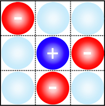
In the mean-field theory, the ionic size effect may be casted by a two dimensional lattice-gas model, as shown in Fig. 2 . Note that figure 2 may be any infinite thin layer parallel to the electrode surface, and the ion/solvent distribution varies from layer to layer in the EDL, while it is constant in the bulk region at infinite distance toward the electrode surface.

Fig. 2.

	Figure Option View Download New Window
	Fig. 2. A two-dimensional representation of the mean field lattice-gas model, in which blue hard spheres represent cations, red hard spheres represent anions, and iceblue hard spheres represent the solvent molecules or empty space for pure ionic electrolyte, such as ILs.

By taking into account ion sizes, Bikerman proposed an EDL model in 1942. ^{[ 9 ]} Bikerman’s model may be easily understood with the lattice-gas scheme in Fig. 2 . Note that the volume is constant for such a system, so that the derivation starts with the Helmholtz free energy, F , of the lattice-gas model,

The underlying assumption of the Bikerman model is the constant total number, i.e.,

The above constraint implies ∂N _s / ∂N _± = −1. Thus, by taking the chemical potential of each kind of ions, i.e., μ _± = ∂F / ∂N _± and using Sterling approximation ln N _± ! = N _± ln, N _± − N _± , we have

Remembering the fact that the chemical potential of each component is equal everywhere for an equilibrium system, i.e., μ _± = μ _∞ , and ϕ _∞ = 0, N _+,∞ = N _−,∞ = N _∞ in the bulk lattice, the numbers of ions in different layers are given by

Note that equation ( 12 ) is correct for any sizes of ions and solvent molecules for the lattice–gas model in Fig. 2 , with constant number constraint in Eq. ( 10 ). In the following derivation, Bikerman took into account the constant volume of each layer, i.e.,

Equation ( 14 ) is re-derived in the lattice-gas scheme, for the reason that Bikerman presented it with no explicit derivation. ^{[ 9 ]} Note that the Gouy–Chapman model can also be derived in a similar manner, with an additional assumption of N _s → ∞, though the original derivations were performed in terms of osmotic or hydrostatic pressure. ^{[ 4 , 5 ]} Thus, the Gouy–Chapman model is often referred to as an infinite dilute model.

Comparing with the Boltzmann distribution in Eq. ( 3 ), we can see that the modified Boltzmann distribution in Eq. ( 14 ) is the consequence of ionic sizes. Thus, instead of infinite c _± , the density at infinite ϕ ₀ in Eq. ( 2 ), which is surpassed in Eq. ( 14 ) by the fractional term. Thus, C _d decreases at high ϕ ₀ with a square-root decay wing. ^{[ 10 ]} Bikerman also pioneered on taking into account the polarizable effects manifested in the dipole moment of the coordinated solvents, ^{[ 9 ]} which is beyond this short review.

From the previous section, it can be seen that the ionic density distribution of the Bikerman model is derived for the ions/solvent molecules of equal sizes. Though equation ( 14 ) does not prevent its further applications on the ions/solvent molecules of different sizes, the inherent inconsistence is imposed by the constant number constrain of EDL. The reason is that the constant number constraint in Eq. ( 10 ) is not consistent with the constant volume constraint in Eq. ( 13 ), except all the ions and solvent molecules have equal sizes. For different sizes, a constant volume constraint means the numbers vary at different EDL. Thus, as pointed out by Freise, ^{[ 11 ]} equation ( 13 ) is more reasonable for the EDL model of asymmetric ions and solvent molecules.

The Freise model can also be understood within the framework of the lattice–gas mean field model in Fig. 2 , with the constant volume constraint by Eq. ( 13 ), which implies that ∂N _s / ∂N _± = − ν _± / ν _s . The derivation follows the Bikerman model in Section 3, and the numbers of ions in different layers are given by

The above expression includes the ionic size effect as comparing to Eq. ( 12 ). For v ₊ = v ₋ = v _s , equation ( 15 ) reduces to Eq. ( 12 ). ^{[ 11 ]} It is notable that N _s in Eq. ( 15 ) should not be obtained by Eq. ( 10 ) for ions/solvent molecules of different sizes, but by Eq. ( 13 ). However, it appears that the Freise model takes Eq. ( 10 ) for N _s , and the ionic density distributions are written as

As discussed above, equation ( 16 ) is derived from Eq. ( 15 ) with constant number constraint by Eq. ( 10 ), thus it is not consistent with the constant volume constraint either. It is of interest to note that equation ( 16 ) was rigorously derived by Freise ^{[ 11 ]} in terms of osmotic pressure, similar to Gouy ^{[ 4 ]} and Chapman, ^{[ 5 ]} instead of the chemical potential as in Section 3. However, it is inappropriate to apply the osmotic pressure to the solvents, and that may cause the inconsistence between Eqs. ( 15 ) and ( 16 ). Since the Bikerman model and the Freise model are very similar, they are called the Bikerman–Freise model. ^{[ 7 ]}

Nevertheless, for v ₊ = v ₋ = v _s = v , equations ( 16 ) and ( 14 ) become equivalent as γ _± = c _± v in this case, and both are correct for the ions/molecules of equal sizes. Indeed, this is a big step on the improvement of the Gouy–Chapman model for the dimensionless ions. For the equal ionic/molecular sizes, the ionic distribution may be written as ^{[ 7 ]}

Thus, the charge density in EDL according to Eq. ( 2 ) is ^{[ 7 , 12 , 13 ]}

Solving the Poisson function in Eq. ( 4 ), and Freise further derived the analytical expression of C _d , i.e., ^{[ 7 , 8 , 10 – 12 , 14 ]}

The above expression was re-discovered many times during the following half century. ^{[ 7 ]} However, even Freise was not the first person to get Eq. ( 19 ). In fact, Stern derived a similar expression of C _d in 1924, ^{[ 6 ]} which was almost forgotten in history, ^{[ 7 , 11 ]} partly due to the glory of the GCS model proposed in the same milestone paper. ^{[ 6 ]}

The omission of the ionic size effect addressed by the Bikerman-Freise model for the following half century is reasonable, because the GCS model can often be applied on the C _d and EDL properties of dilute electrolyte reasonably well. With the development of ILs since 2000, the capacitance properties of this new kind of room temperature molten salts have caught a great deal of attention. Interestingly, it is often found that C _d curves of ILs are bell-shaped, in contrast to the traditional parabola-shaped C _d at low applied potential. ^{[ 10 , 12 , 14 ]}

In 2007, Kornyshev ^{[ 10 ]} and Kilic, Bazant, and Ajdari ^{[ 12 ]} independently published two papers on the EDL of equally sized ions. While Bazant et al. ^{[ 12 ]} orientated on the strong electrolyte system for the diffusion process, Kornyshev ^{[ 10 ]} specifically orientated toward ILs for the differential capacitance, C _d . Both works are based on the mean field lattice-gas model as shown in Fig. 2 , and derived the analytical expression of C _d , which is essentially the same as Eq. ( 19 ) by Freise, as expected. It is of interest to note that both works were stimulated by Borukhov, Andelman, and Orland, ^{[ 15 ]} which is actually another example of the re-discovery of the Bikerman–Freise model, and it appears that Freise’s work was not realized by either of these authors.

In Kornyshev’s well-celebrated work, ^{[ 10 ]} the effects of ionic size on C _d of ILs are vividly described by γ _∞ defined by Freise. ^{[ 11 ]} Since ions are equally sized with the same volume v ₊ = v ₋ = v , equations ( 10 ) and ( 13 ) are equivalent, so that the molar fraction of individual ion in the bulk is

Thus, in Kornyshev’s derivation, the term 4 c _∞ v in Eq. ( 19 ) is replaced by 2 γ . ^{[ 10 ]}

The significance of γ may be illustrated by Fig. 2 for the bulk lattice. For γ = 1, all the lattices are completely occupied by the ions. For γ → 0, equation ( 19 ) reduces to the Gouy–Chapman model, as discussed in Section 4. For γ > 0, then all the lattices are partially occupied by the ions. Thus, counterions cannot approach the electrode with infinite density, but instead “crowding” at the interface and may extend several EDL layers at high electrode potential. Such an effect manifests in Eq. ( 19 ) by taking the high ϕ ₀ limit with

The above expression of C _d for the high ϕ ₀ limit was first given by Kornyshev ^{[ 10 ]} to the authors’ best knowledge, though such inverse-square-root decay of C _d on the high ϕ ₀ was indicated by Bikerman. ^{[ 9 ]}

By taking the low ϕ ₀ limit, equation ( 19 ) may be written as ^{[ 10 ]}

It can be clearly seen from Eq. ( 23 ) that C _d increases with ϕ ₀ for γ < 1/3 at low ϕ ₀ and results in an overall camel-shaped C _d , while it monotonically decreases with ϕ ₀ for γ > 1/3 and results in an overall bell-shaped C _d . Equation ( 19 ), as well as its high ϕ ₀ and low ϕ ₀ behavior, has been verified by many recent experiments and simulations on the C _d of ILs. ^{[ 14 ]} Thus, Kornyshev’s work in 2007, ^{[ 10 ]} though it represented another re-discovery of the Bikerman–Freise model, stimulated tremendous interest in the development of EDL theory for the pure ionic electrolytes.

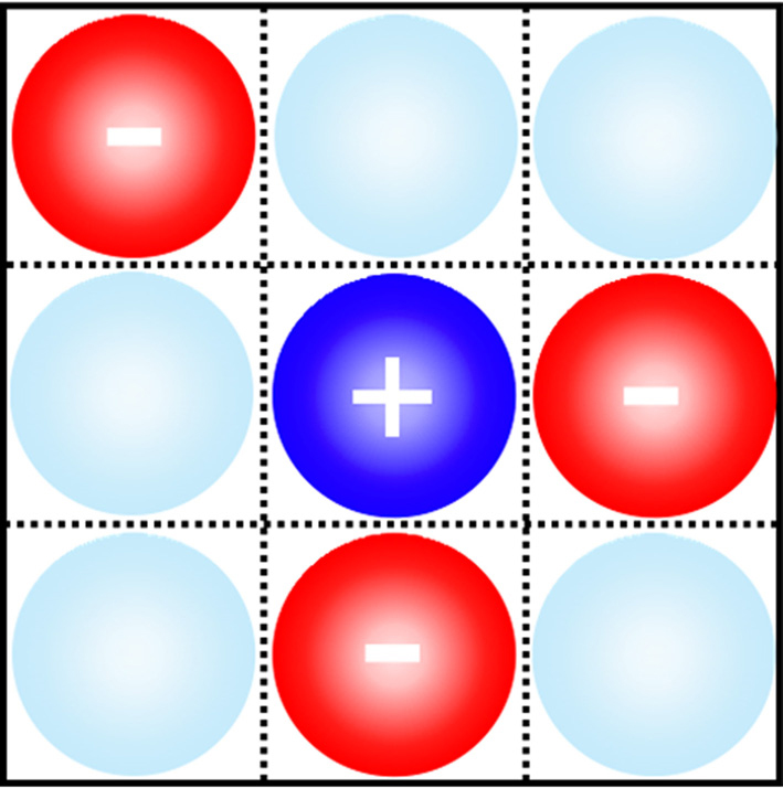
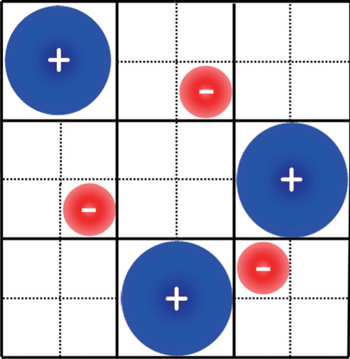
It should be addressed that C _d in Eq. ( 19 ) was derived explicitly for the symmetric ions of equal sizes. For asymmetric ions with different cation and anion sizes, that is, v ₊ ≠ v ₋ , the lattice–gas model can be represented by Fig. 3 , in which an obvious fact is that the compressibilities of cations and anions are different. Thus, for asymmetric ions of different compressibilities, γ ₊ ≠ γ ₋ , Kornyshev proposed the semi-empirical u ₀ -dependent γ as ^{[ 10 ]}

Fig. 3.

	Figure Option View Download New Window
	Fig. 3. A two-dimensional representation of the mean field lattice–gas model for ILs, in which blue hard spheres represent cations, and red hard spheres represent anions. The space is divided into lattices by the solid line to accommodate cations, and then subdivided by dotted line to accommodate anions, in order to take into account different cationic and anionic sizes.

For the lattice-gas model in Fig. 3 of asymmetric ions of volume ratio ξ = v ₋ / v ₊ = γ ₋ / γ ₊ , Han et al . attempted to get the partition function via two steps, i.e., Ω = Ω ₊ Ω ₋ . For the total available lattices N that are capable of accommodating cations N ₊ , and the left are for anions, ( N − N ₊ )/ ξ . Based on the above consideration, the partition function of the lattice-gas model in Fig. 3 may be written as ^{[ 8 ]}

Following the derivation in terms of the Helmholtz free energy in Section 3, the charge density is given by ^{[ 8 ]}

It can be shown that as ξ = 1 the above equation reduces to Eq. ( 18 ), using the relations sinh (e ϕ ₀ / kT ) = [exp( eϕ ₀ / kT ) − exp (− eϕ ₀ / kT )]/2 and sinh ² ( eϕ ₀ /2 kT ) = [exp( eϕ ₀ / kT ) + exp (− eϕ ₀ / kT ) − 2]/4. In the ϕ → 0 limit, using the first order approximations, it can be shown that Eq. ( 26 ) reduces to

From the above approximation, it can be seen that for asymmetric ions ξ < 1, the EDL charge density may well exceed that of the dimensionless ion predicted by the Gouy–Chapman model in Eq. ( 3 ) or the Bikerman–Freise model in Eq. ( 18 ), which give ρ ≈ −2 c _∞ e ² ϕ / kT in the ϕ → 0 limit. Such an effect is amplified as ξ → 0 and γ → 1. ^{[ 8 ]}

Solving the Poisson equation ( 4 ) with charge density in Eq. ( 26 ), the analytical C _d in the SAMFT model is ^{[ 8 ]}

Though the above C _d in the SAMFT model looks complicated, it is inherent from the Gouy–Chapman and Bikerman–Freise models. As can be seen that equation ( 28 ) reduces to Eq. ( 19 ) for ξ = 1, which further reduces to Eq. ( 5 ) in the γ → 0 limit. Also, the high ϕ ₀ limit of Eq. ( 28 ) gives ^{[ 8 ]}

Remembering that γ ₊ = γ and γ ₋ = ξγ , the above inverse-square-root decay is consistent with Eq. ( 22 ) for the symmetric ions of ξ = 1, but includes a “crowding” effect for the positive polarization branch and negative polarization branch characterized by the size of counter ions in the high ϕ ₀ wing.

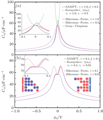
At low electrode potential ϕ ₀ , the C _d of the Gouy–Chapman theory in Eq. ( 5 ) imposes the upper limit of the Kornyshev model ^{[ 10 ]} and the Bikerman–Freise model ^{[ 9 , 11 ]} in Eq. ( 19 ) either with semi-empirical potential-dependent γ ( u ₀ ) or with constant γ in Eq. ( 24 ), as shown in Fig. 4(a) . On the other hand, this is not the case for Eq. ( 28 ). With decreasing γ , both Eqs. ( 19 ) and ( 28 ) approach asymptotically Eq. ( 5 ) from the upper and lower sides.

Fig. 4.

Figure Option View Download New Window

Fig. 4. C d at different levels of theory. (a) C d by Eq. ( 28 ) with γ = 1.0, ξ = 0.5 (black), Eq. ( 19 ) with semi-empirical γ ( ϕ 0 ) in Eq. ( 24 ) for γ + = γ = 1.0 and γ − = ξγ = 0.5 (red), Eq. ( 19 ) with γ = 1.0 (blue) and γ = 0.5 (pink), with Eq. ( 5 ) (green). (b) C d by Eq. ( 28 ) with γ = 0.1, ξ = 0.1 (black), Eq. ( 19 ) with semi-empirical γ ( ϕ 0 ) in Eq. ( 24 ) for γ + = γ = 0.1 and γ − = ξγ = 0.01 (red), Eq. ( 19 ) with γ = 0.1 (blue) and γ = 0.01 (pink). Insets in (a) and (b) are C d at different levels of theory between potentials of −0.1 to 0.1 V.

Considering asymmetric ionic liquids, the C _d at the negative branch obtained by Kornyshev using the semi-empirical Eq. ( 24 ) with Eq. ( 19 ) for γ ₊ = 1.0 and γ ₋ = 0.5 is consistent with the Bikerman–Freise model ( γ = 1.0 and γ = 0.5), while that at the positive branch agrees well with the Bikerman–Freise model for γ = 1.0. It should be mentioned that the C _d at the potential of zero charge (PZC) predicted by the SAMFT model can be higher than the Debye capacitance, with C _d in the other models equal the Debye capacitance.

The C _d curves become camel-shaped for the Kornyshev model ^{[ 10 ]} for γ ₊ = 0.1 and γ ₋ = 0.01 and the Bikerman–Freise model ^{[ 9 , 11 ]} for γ = 0.1 and γ = 0.01 in Fig. 4(b) . Comparing the four curves in Fig. 4(b) , it can be seen that the values of C _d of the SAMFT model are closer to the results by the Bikerman-Freise model than the Kornyshev model with semi-empirical potential-dependent γ ( u ₀ ) or with constant γ . Meanwhile, the Bikerman–Freise model, Kornyshev model and SAMFT model successfully predict the inverse-square-root law resulted from “crowding” of counter ions. Such a crowding phenomenon of counterions, as shown in the illustration of Fig. 4 , may increase the thickness of the compact layer or Stern layer and decrease the capacitance.

In this article, we briefly reviewed the development of the mean field based EDL theory from the Helmholtz model to the SAMFT model. Though the effects of the ionic size on the EDL and C _d was studied by the Bikerman–Freise model more than half a century ago, the re-discovery of this theory was experimentally called by the new electrolyte materials, ILs. ^{[ 10 ]} Based on these efforts, the SAMFT model further provides a C _d for asymmetric 1:1 IL in Eq. ( 29 ), which reduces to the Bikerman–Freise model, and the Gouy–Chapman model for dimensionless ions.

It should be noted that the lattice-gas models presented in Figs. 2 and 3 vary with the distance to the electrode surface and electrode potential. Furthermore, the lattice-gas model is actually two-dimensional and is inifinite thin along the electrode surface normal direction, in order to apply the continuous differentiation with a one-dimensional Poisson equation ( 4 ). As a matter of fact, this is an inherent limitation of mean field theory for the analytical expressions. This inconsistence of sized ions may be remedied by a series of a Stern layer, as has been applied by Kornyshev for the extended Bikerman–Freise model. ^{[ 16 ]}

Finally, we mentioned that the current review only focussed on mean field EDL theory. The benefit is that the analytical expressions can often be derived, and such a simple model can often help to understand the complex experimental results in a qualitative manner with a vivid picture. Of course, the mean field based EDL theory oversimplified the real situation. For example, overscreening, or charge inversion effect, caused by the correlations between cations and anions, cannot be treated by the mean field framework. For the latter, density functional theory and computer simulations that are well beyond the scope of this article, can often be applied to get more realistic results, though the analytical expressions are lost with simple pictures.