Two kinds of generalized gradient representations for holonomic mechanical systems
[Mei Feng-Xiang 1 , Wu Hui-Bin 2, †,  ]
]
]
|
|


† Corresponding author. E-mail:
Project supported by the National Natural Science Foundation of China (Grant No. 11272050).
Two kinds of generalized gradient systems are proposed and the characteristics of the two systems are studied. The conditions under which a holonomic mechanical system can be considered as one of the two generalized gradient systems are obtained. The characteristics of the generalized gradient systems can be used to study the stability of the holonomic system. Some examples are given to illustrate the application of the results.
In Ref. [ 1 ], it was pointed out that the gradient system is especially suitable for study by using the Lyapunov function. Reference [ 2 ] indicated that there are the skew-gradient system, the gradient system with a symmetric negative definite matrix, the gradient system with a negative semidefinite matrix, and so on, in addition to the general gradient system. References [ 3 ] and [ 4 ] demonstrated that an autonomous ordinary differential equation has a first integral if and only if it can be written as a skew-gradient system, which provides a general way to rewrite such a system as a skew-gradient system, and from which several new integral-preserving discrete gradient methods are constructed. Reference [ 5 ] studied the skew-gradient representation for autonomous stochastic differential equations with a conserved quantity, from which direct/indirect discrete gradient approaches are constructed. Some results have been obtained in the research of the relation between constrained mechanical systems and gradient systems. [ 6 – 18 ] However, in those studies, the matrix or the function of the gradient system has no time t . When its matrix or function contains time t , the system can be called a generalized gradient system. There are two types of generalized gradient systems that are particularly useful for the study of stability. One is the generalized skew-gradient system, and the other is the generalized gradient system with a symmetric negative definite matrix. In this paper, we will transform the holonomic mechanical system into the two kinds of generalized gradient systems under certain conditions, then discuss the stability of solution of the mechanical system by using the property of the generalized gradient system.
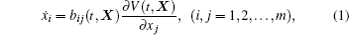
The differential equations of the generalized skew-gradient system have the form
Taking the derivative of V with respect to time, according to Eq. (

If V can be a Lyapunov function, i.e., it is positive definite and satisfying ∂V / ∂t < 0, then the solution of system (
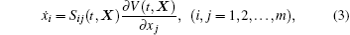
The differential equations of the system have the form
Taking the derivative of V with respect to time, according to Eq. (

The differential equations of a general holonomic system in the generalized coordinates have the form

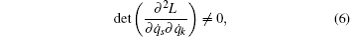
Suppose that the system is nonsingular, namely,

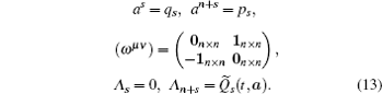
Let


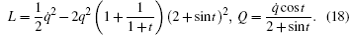
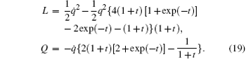
By introducing the generalized momentum p s and the Hamiltonian H ,


Here Q̃ s are the generalized forces Q s written in canonical variables.
Generally speaking, equations (


For Eq. (


It is worth noting that, if conditions (
For the general holonomic system in the generalized coordinates, if it can be transformed into the generalized gradient system (
We transform it into a generalized gradient system and discuss the stability of zero solution.
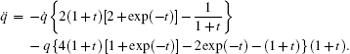
Equations (

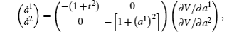
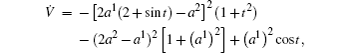
If let


It also has the following matrix form:


It is a generalized skew-gradient system (1). Function V is positive definite in the neighborhood of a 1 = a 2 = 0, and

Therefore, zero solution a 1 = a 2 = 0 is stable.
We transform it into a generalized gradient system and discuss the stability of zero solution.
Equations (
Let


It also has the following matrix form:


It is a generalized gradient system (

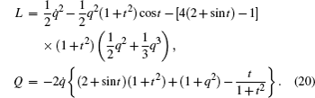
We transform it into a generalized gradient system and discuss the stability of zero solution.
Equations (
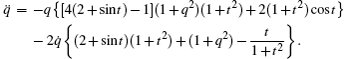
Let


It also has the following matrix form:

It is a generalized gradient system (
The stability problem of non-constant mechanical systems is important and difficult. It is often not easy to construct the Lyapunov function directly from the differential equations. In this paper, we have studied two kinds of generalized gradient representations for general holonomic mechanical systems. When a system has been transformed into a generalized gradient system, one can discuss the stability of solution of the mechanical system by using the property of the generalized gradient system. If the system is rewritten in the generalized skew-gradient system (
| 1 | |
| 2 | |
| 3 | |
| 4 | |
| 5 | |
| 6 | |
| 7 | |
| 8 | |
| 9 | |
| 10 | |
| 11 | |
| 12 | |
| 13 | |
| 14 | |
| 15 | |
| 16 | |
| 17 | |
| 18 |