Data point selection for weighted least square fitting of cavity decay time constant
He Xing 1, 2, 3 , Yan Hu 1, 2, 3 , Dong Li-Zhi 1, 2 , Yang Ping 1, 2 , Xu Bing 1, 2, †,
Laboratory on Adaptive Optics, Institute of Optics and Electronics, Chinese Academy of Sciences, Chengdu 610209, China
Key Laboratory on Adaptive Optics, Chinese Academy of Sciences, Chengdu 610209, China
University of the Chinese Academy of Sciences, Beijing 100039, China


† Corresponding author. E-mail: bing xu ioe@163.com

Project supported by the Preeminent Youth Fund of Sichuan Province, China (Grant No. 2012JQ0012), the National Natural Science Foundation of China (Grant Nos. 11173008, 10974202, and 60978049), and the National Key Scientific and Research Equipment Development Project of China (Grant No. ZDYZ2013-2).

Abstract
Abstract

For the accurate extraction of cavity decay time, a selection of data points is supplemented to the weighted least square method. We derive the expected precision, accuracy and computation cost of this improved method, and examine these performances by simulation. By comparing this method with the nonlinear least square fitting (NLSF) method and the linear regression of the sum (LRS) method in derivations and simulations, we find that this method can achieve the same or even better precision, comparable accuracy, and lower computation cost. We test this method by experimental decay signals. The results are in agreement with the ones obtained from the nonlinear least square fitting method.

1. Introduction

The cavity ring-down (CRD) technique is a sensitive detection technique for measuring weak absorption [ 1 ] or high reflectivity. [ 2 ] The laser beam, pulsed or continuous, is firstly coupled into a ring-down cavity (RDC). After the laser pulse is injected or the continuous wave is suddenly shut off, the intensity of the output optical signal of RDC, I , will decay exponentially with time t , [ 1 ]

Here, A is the initial amplitude, offset refers to the combination of background noise and instrumental offset, and τ is the cavity decay time which has a relationship with RDC round-trip loss δ , as indicated as follows: [ 3 ]

where L corresponds to the cavity length, which can be measured directly, c is the speed of light, α ( λ ) is the optical loss caused by weak absorption, R m ( λ ) is the reflectivity of the m -th cavity mirror, and γ corresponds to other losses that result from diffraction or scattering, etc. For the accurate δ is essential for the calculation of weak absorption or high reflectivity, it is nontrivial to ensure the accuracy of extracted cavity decay time.

There are a lot of extraction methods adopted in the CRD technique, including the nonlinear least square fitting (NLSF) algorithm [ 4 7 ] such as the Levenberg–Marquardt (LM) algorithm, the weighted least square (WLS) method, [ 5 , 8 ] and the extractions based on Fourier transform (FT) [ 9 , 10 ] or linear regression of sum (LRS) [ 11 ] of the decay signal, etc. Their extraction performances have been analyzed and compared by several papers [ 12 15 ] where the extraction precision, accuracy, and computation cost of each method were comprehensively considered. Their analyses indicated the NLSF method can achieve the finest precision. However, the computation cost of the NLSF method may be a little high because it increases usually with the increase of iterations, so references [ 14 ] and [ 15 ] both recommended the LRS (also known as corrected successive integration, CSI) method to extract the cavity decay time finally. They found that the LRS method can achieve comparable extraction performance with the NLSF method, [ 14 , 15 ] which is its main advantage over the WLS and FT methods. Besides, the LRS method takes lower computation cost than the WLS method. [ 14 ] However, we find that the extraction performance of the WLS method is highly related to the number of data points. By selecting proper data points for fitting, the WLS method can achieve fine performance and low computation cost simultaneously. The main drawback of the WLS method is that it is sensitive to offset. It is thought that nonzero offset brings deviation because the logarithm of the decay signal is nonlinear; whereas zero offset results in information loss when calculating the logarithms of negative data points. [ 5 ]

In this paper, we focus on the effect of offset and explore it from the calculation procedure of the WLS method. We find that the WLS method needs data point selection in theory, so we supplement a theoretical data point selection to the common WLS method. This improved method is referred to as the WLS-DS method. Its expected precision, accuracy, and computation cost are also derived. According to these derivations and the corresponding simulations, we find the WLS-DS method can actually take a lower computation cost than the LRS and the NLSF methods to achieve the comparable or nearly the same fitting performance. Finally, we test the WLS-DS method by actual decay signals of an optical feedback cavity ring-down (OF-CRD) [ 16 , 17 ] setup.

2. Theory
2.1. Data point selection for the WLS method

If there is no excitation of the multiple cavity mode, the decay signal of RDC will be monoexponential. After recording and digitalizing, the decay signal S can be given by

Here, τ is the cavity decay time, a is the reciprocal of τ , i.e., a = 1/ τ , the subscript i = 1, …, N , N is the number of data points, and then, the natural logarithm of S i is taken as [ 1 ]

The effect of offset i is processed by subtracting the mean value of offset, [ 1 ] that is

The last term of Eq. ( 5 ) indicates that the effect form of offset to data point is very complicated. However, this term can be simplified according to ln(1 + x ) ≈ x (when ❘ x ❘ ≪ 1) if this data point ensures that the corresponding fraction part of the last term is far less than one. It must be noticed that neither A nor a in the denominator can be known beforehand, so we have to give them initial guess values, noted as A 0 and a 0 , as shown in Eq. ( 6 ),

Equation ( 6 ) indicates that a selection of data points is actually indispensable for the WLS method. These selected data points approximately suffer an exponential effect caused by the offset. If these data points are weighted by exp(− a 0 t i ) (in the WLS method, this weight will be squared as exp(−2 a 0 t i ) after the linear least algorithm [ 5 , 8 ] ), they can suffer an identical effect from the offset. Thus, the residual of the offset can be processed as a constant, that is

Traditionally, this constant is set to be zero to eliminate the deviation caused in linearization. [ 1 , 5 ] However, we find this constant can also be set to be a positive value b , provided that the following inequality holds:

Thus

where D i refers to

Here, we can see that b provides us with a reference point by which we can select proper signal data points for WLS fitting. In this way, we find a condition of selecting data points, which can help us truncate the optimal data point interval according to the decay signal transient itself. It should be noticed that offset i is unknown beforehand, so we must execute the data point selection in consideration of the total decay signal, that is, the data points selection depends on

Generally, the selected data points are positive, so we need not worry about the information loss. In addition, equation ( 11 ) implies an instructive method to determine the value of b (the value of k must be far less than 1 so it is usually set directly in advance), which can be derived by simply rearranging Eq. ( 11 ),

Here, we can see that b is not very large unless the signal initial amplitude A 0 is large enough. These data points are rearranged as Eq. ( 9 ) and analyzed by the linear least square algorithm. Then the final expression of fitted a can be written as

Here, K is the total number of selected data points, W j corresponds to the weight factor exp(− a 0 t j ), and the subscript fit means this parameter is a calculated one. In CRD measurement, τ fit is more commonly used, which is the reciprocal of a fit .

In the WLS-DS method, the information loss caused by zero offset can be expected to be mitigated because there are fewer or even no negative data points in fitting, meanwhile the deviation of nonzero offset is limited by the data point selection based on Eq. ( 8 ). The data point selection method stems from the underlying linear approximation condition rather than an empirical value, which is usually adopted in previous linear least square (LS) fitting, such as t ≈ 3 τ . [ 4 , 5 ] Compared with the previous LS method, the WLS-DS method only selects those data points which can retain their information as much as possible for fitting, so it can theoretically achieve more accurate results.

2.2. Assessments of the WLS-DS method

An extraction method (even an improved one) should be assessed by three requirements which are precision, accuracy, and computation cost. [ 12 , 14 ] A noticeable point is that these requirements are not mutually independent of each other. In fact, they are all related to the number of data points, N or K here. We should not ignore this point in the following assessments and comparisons.

As indicated in Ref. [ 12 ], a Δ t ≪ 1 and f Δ t ≈ 1, where f is the reciprocal of the systemic response time t f and Δ t is the time interval of data acquisition, are required by a CRD system. As for our CRD system, Δ t is 12.5 ns (80 MS/s sampling) and t f has been measured by Gong and Li [ 18 ] that was less than 20 ns. The typical a of our CRD system is in a range of (0.5 − 1) × 10 6 s −1 which corresponds to 1–2 μs cavity decay time. Both of these hardware limitations are met. If we further assume that σ , the standard deviation value of offset, is constant, we can make our derivations in the following.

At first, we must notice that A 0 and a 0 should be regarded as independent constants in the WLS-DS method, and b is a preset parameter. Under these conditions, we can write the expression of expected precision of a fit according to error propagation [ 19 ]

For concise description, we define three constants as

Then the partial derivative of D j can be written as

and σ 2 ( D j ) after data point selection can be approximately given by

Thus, we can obtain the simplified expression of expected precision

Take our typical laboratory case for example, where τ is 1.2 μs, A is 1 V, and σ = 4 mV. If we set b = 0.5 mV, and k =0.01, the calculated K is 287 and σ ( a fit ) = 1005 s −1 which corresponds to ± 1.45 ns precision. We test this result by a simulation which contains 5000 decay signals, the statistical result is 1.19975 ± 0.00146 μs. The precision is ± 1.46 ns, quite close to the derived value.

To find the relations between σ 2 ( a fit ) and those method parameters, such as a , A , Δ t , etc., we let K approach to infinity meanwhile a Δ t approaches to zero to obtain the following equation:

We can see that σ 2 ( a fit ) is nearly proportional to a 3 and Δ t , while nearly inversely proportional to A 2 .

Then, we analyze the expected fitting bias by the method introduced by Lehmann and Huang. [ 12 ] In Eq. ( 9 ), if the second-order term in the Taylor expansion of D i is reserved, we can obtain

Actually, the last term on the right-hand side of Eq. ( 20 ) is just the source of bias. The numerator of this term has an ensemble average value of

As a Gaussian-distributed variable, ⟨offset 2 ⟩ = σ 2 . Thus, we can deduce the ensemble average value of the last term on the right-hand side of Eq. ( 20 ), which is denoted as

Combining Eq. ( 22 ) with Eq. ( 13 ), we can write the expected bias

If we assume that there is no initial guess error, i.e., A 0 = A and a 0 = a , equation ( 23 ) can be simplified into

Because Δ a fit is positive, the fitted τ of the WLS-DS method is always smaller than the real value.

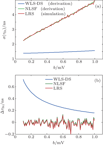
Based on Eqs. ( 18 ) and ( 24 ), we can calculate the fitting precision and fitting accuracy of τ fit , which are noted as σ ( τ fit ) and Δ τ fit , correspondingly. To test the above derivations, we made a simulation where τ is 1.2 μs, A is 1 V, and σ = 4 mV. We fix k to be 0.01 and let b range from 0.1 mV to 1 mV. The statistical results of five thousand decay signals are illustrated in Fig. 1 . We can see that the derivations are basically in agreement with the simulations. We can also find that the fitting precision and fitting accuracy have contrary dependences on b , which means the WLS-DS method cannot achieve high precision nor find accuracy simultaneously. Hence, we make another comparison as shown in Fig. 2 to determine whether the performances of the WLS-DS method can meet the actual measurements.
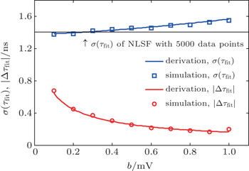
Fig. 1. Comparisons between derivations and simulations of expected precision and accuracy. When b = 0.2 mV (corresponding to K = 375), the precision of the WLS-DS method is better than that of the NLSF method with 5000 data points (the solid black line in Fig. 1 ) which are calculated according to the derivation of Ref. [ 12 ].
Fig. 2. Comparisons of the WLS-DS method with the NLSF and the LRS methods. In panel (a), the NLSF and the LRS methods are both executed by using the selected data points of the WLS-DS method. The derivation of NLSF precision in panel (a) has been achieved by Ref. [ 12 ]. However, for the LRS method, its precision and accuracy are too complicated to give closed forms, [ 12 ] so our presentation of the LRS method is based on simulations. Y -axes in panels (a) and (b) are in different ranges, which indicates Δ τ fit is smaller than σ ( τ fit ).

The comparisons of performances are given in Fig. 2 . The accuracies of NLSF and LRS methods are obtained by simulations which contain 5000 decay signals in each case. The largest relative bias of the WLS-DS method is less than 0.06%, whereas the smallest relative bias is about 0.015%, which is still worse than those of the NLSF and LRS methods. Although the WLS-DS method shows a slightly worse accuracy than those of the other two methods, it achieves quite fine precision in very few data points. For example, in the typical case of our lab, the NLSF method needs 2243 data points to achieve the precision of ± 1.45 ns, which is calculated according to the derivation in Ref. [ 12 ], while the LRS needs about 880 data points to achieve its best precision which is only ± 1.72 ns (obtained by simulation). Besides, we should notice that for the fitting result, its bias is always less than its dispersion, which is a measure of precision. So we think that the accuracy of the WLS-DS method is acceptable if we choose proper b . Generally, b can be as large as possible to obtain fine accuracy.

Finally, the computation cost of the WLS-DS method is also considered. It seems that more than 10 multiplications and 7 additions per data point are needed at a glance of Eq. ( 13 ). However, we must notice that A 0 and b are both preset; meanwhile the series W and t can also be known before the fitting. Therefore, most calculations can be simplified by the summation formula of the geometric series except these two terms which contain D j . For clearer presentation, we give the following equivalent form of Eq. ( 13 ):

Here,

We can see that the required number of floating point calculations is on the order of 3 K multiplications (the W 2 and W K are just regarded as calculations of exponential function) and 2 K additions. In fact, the main computation cost is taken in the logarithmic calculation of D j . As far as we know, the most efficient equivalent series of a logarithm is [ 20 ]

Here, x > 0 can be ensured by the data point selection procedure. We find that this serial converges very fast only when x ≈ 1. However, the discussed x , i.e., the amplitude of data point, may be very small in fact, so we recommend the following function for the logarithm calculation: [ 20 ]

This expansion stops when

Here, e is the base of the natural logarithm, and y is a certain number to make e y x ≈ 1. In addition, taking the former simulation for example, the logarithms of data points are calculated according to Eq. ( 28 ) and a logarithm function package. If the amplitude of data point S i is in a range of (0.8–1), y is set to be zero; while if S i is in a range of (0.2–0.8), y is set to be one; otherwise y is set to be two. If e is set to be 2.718282, the WLS fitting based on Eq. ( 28 ) gives 1.19990 ± 0.00137 μs. Whereas the WLS fitting based on the logarithm function package gives 1.19986 ± 0.00137 μs. The relative difference is less than 0.005% meanwhile the computation cost is less than 15 K. Thus, we think that the computation of the WLS-DS method can be limited in 20 K floating point calculations if we use an efficient enough code.

The computation costs of the NLSF and the LRS methods have been derived by Lehmann and Huang. [ 12 ] They found that at least 6 floating point calculations (3 additions and 3 multiplications) are needed for a single data point in the NLSF extraction, and at least 13 floating point calculations (8 additions and 5 multiplications) are needed for a single data point when using the LRS method. However, these two methods need more data points to achieve a fine fitting performance. In the typical case of our laboratory, the computation costs of these three methods to achieve the precision of 1005 s −1 (±1.45 ns) are presented in Table 1 .

Table 1.

Comparisons of computation cost among NLSF, the LRS, and the WLS-DS methods.

.

We can see the computation cost of the WLS-DS method is lower than those of the NLSF and LRS methods.

Let b approach to zero, we can achieve the common WLS fitting. Combining former derivations and the tendency of the WLS-DS method in Fig. 2 , we can deduce that the WLS method has a little better precision but a much more obvious bias. Furthermore, its computation cost is also higher than that of the WLS-DS method.

3. Experiments and results

Our experimental OF-CRD setup is presented in Fig. 3 . A CW F–P diode laser (Power Technologies, IQ1A07) of 1060 nm was adopted as a light source. Its output signal was modulated by a 100-Hz square wave generated by a waveform generator (Spectrum, M2i.6021). A folded cavity composed of three mirrors (M 1 , M 2 , and M 3 ) with a high reflectivity coating was used as the RDC. M 1 and M 2 are two identical plano-concave mirrors each with a curvature radius of 1 m, and M 3 is a plane mirror. By properly modulating the intensity of retro-reflected light from the RDC, the optical feedback could achieve line-width narrowing and frequency locking to the semiconductor laser, [ 16 , 17 ] so the coupling between the laser beam of the light source and the RDC could be easier to achieve. At the fall step of the square wave, the light source was switched off suddenly and the RDC decay transient began from a certain initial amplitude. The output signal of the RDC was focused on an InGaAs PD (Thorlabs, PDA400) by the lens L 1 . A data acquisition (DAQ) card (Spectrum, M2i.3010, 80MSample/s, 12 bit) was employed to acquire the data from PD. The acquisition started at the fall step of the square wave at the time when the decay transient began and then transferred the data to the PC for subsequent analyses. In this setup, an He–Ne laser and two plano mirrors M 4 and M 5 were used for conveniently aligning the system.
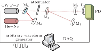
Fig. 3. Schematic setup of the OF-CRD system. The dot lines are light paths, and the solid lines are signal paths.

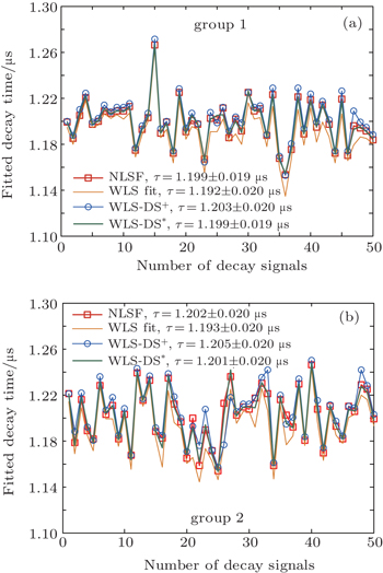
Two groups of 50 decay signals were recorded and analyzed by the NLSF method (the LM algorithm was applied here), the common WLS method, and the WLS-DS method respectively. Here, the NLSF method was chosen as the standard because the LM algorithm has been regarded as the defacto standard in the CRD technique. [ 9 ] The theoretical value of the decay time constant is dependent on the incident angle of M 3 , so it is hard to know beforehand, but it can be approximately determined to be 1.2 μs according to our former experiments. Therefore, the initial guess τ was set to be 1.2 μs, A 0 was set to be a maximum of the decay signal, and offset was calculated beforehand by averaging the tails of several decay signals. Each original decay signal was truncated so only 4000 data points were contained. The mean value of the initial amplitude of decay signals was 0.938 V; statistics indicated that the background offset was 0.019 ± 0.004 V. According to the former simulations, we deduced that the WLS-DS method could give almost the same precision as the NLSF algorithm; meanwhile the accuracy was also comparable. The fitting results are shown in Fig. 4 and statistic results are noted in the legend of each figure.

As detailed in Fig. 4 , data point selection is very helpful for the accuracy of the WLS method. For the WLS-DS method and the NLSF algorithm, both of their statistical results and trends of curves accord with each other very well, especially in the case of b = 1 mV and k = 0.01. Although a theoretical bias of the WLS-DS method exists as shown in Fig. 2(b) , it is not very serious in actual applications. However, for the common WLS method, the difference in statistical result was obvious and the deviation of the curve trend was distinguishable, the only satisfactory point was that it achieved the same fitting precision. The comparison of computation cost is presented in Table 2 , from which we can find that the computation cost of the WLS-DS method is quite low.

Fig. 4. Fitting results of experiment. There are two notes in this figure. Note that the + means that the results of this curve are obtained by the WLS-DS method with b = 0.5 mV and k = 0.01 (blue lines). Note * means that the results of this curve are obtained by the WLS-DS method with b = 1 mV and k = 0.01 (green lines). The WLS fit is corresponding to the common WLS method which uses the total decay signal to fit. (a) Group 1, (b) group 2.
Table 2.

Comparisons of data point number for cavity decay time extraction.

.

Comparable fitting performance with the NLSF algorithm was obtained for the WLS-DS method. Furthermore, former derivations and simulations prove that the WLS-DS method takes a lower computation cost in fact. With this obvious improvement, the WLS-DS method, one of the advanced linear fitting methods, can be a potential high accuracy and fine precision decay time extraction method in the CRD technique.

4. Conclusions

In this paper, a WLS-DS method of extracting the cavity decay time is introduced by deducing the calculation procedures of the WLS method. With a theoretical data point selection procedure contained, it can mitigate the effect brought by the system noise and the instrumental offset to achieve a high accuracy result. After comparing with the NLSF algorithm and LRS method by derivations and simulations, we find that this method can obtain the same or even better precision and comparable accuracy in lower computation cost. The WLS-DS method can be a convenient and useful data processing approach in the CRD technique; furthermore, with its advantage of low computation cost, it could play a more important role in the real-time CRD system.

Reference
1 O’Keefe A Deacon D A G 1988 Rev. Sci. Instrum. 59 2544
2 Anderson D Z Frisch J C Masser C S 1984 Appl. Opt. 23 1238
3 Spence T G Harb C C Paldus B A Zare R N Willke B Byer R L 2000 Rev. Sci. Instrum. 71 347
4 Naus H van Stokkum I H M Hogervorst W Ubachs W 2001 Appl. Opt. 40 4416
5 von Lerber T Sigrist M W 2002 Chem. Phys. Lett. 353 131
6 Kallapur A G Boyson T K Petersen I R Harb C C 2011 Opt. Exp. 19 6377
7 Huang H F Lehmann K K 2011 J. Phys. Chem. A 115 9411
8 Romanini D Lehmann K K 1993 J. Chem. Phys. 99 6287
9 Boyson T K Spence T G Calzada M F Harb C C 2011 Opt. Exp. 19 8092
10 Mazurenka M Wada R Shillings A J L Butler T J A Beames J M Orr-Ewing A J 2005 Appl. Phys. B 81 135
11 Everest M A Atkinson D B 2008 Rev. Sci. Instrum. 79 023108
12 http://www.researchgate.net/publication/251875562_Optimal_Signal_Processing_in_Cavity_Ring-Down_Spectroscopy
13 Istratov A A Vyvenko O F 1999 Rev. Sci. Instrum. 70 1233
14 Fuhrmann N Brühach J Dreizler A 2014 Appl. Phys. B 116 359
15 Wang D Hu R Z Xie P H Qin M Ling L Y Duan J 2014 Spectroscopy and Spectral Analysis 34 2845 (in Chinese)
16 Morville J Romanini D 2002 Appl. Phys. B 74 495
17 Gong Y Li B C Han Y L 2008 Appl. Phys. B 93 355
18 Gong Y Li B C 2007 Proc. SPIE 6720 67201E-1
19 http://en.wikipedia.org/wiki/Propagation_of_uncertainty
20 http://en.wikipedia.org/wiki/Logarithm