Stationary entanglement between two nanomechanical oscillators induced by Coulomb interaction
Wu Qin 1, 2 , Xiao Yin 1 , Zhang Zhi-Ming 1, †,
Guangdong Provincial Key Laboratory of Nanophotonic Functional Materials and Devices (SIPSE), Guangdong Provincial Key Laboratory of Quantum Engineering and Quantum Materials, South China Normal University, Guangzhou 510006, China
School of Information Engineering, Guangdong Medical University, Dongguan 523808, China


† Corresponding author. E-mail: zmzhang@scnu.edu.cn

Project supported by the Major Research Plan of the National Natural Science Foundation of China (Grant No. 91121023), the National Natural Science Foundation of China (Grant Nos. 61378012, 60978009, and 11574092), the Specialized Research Fund for the Doctoral Program of Higher Education of China (Grant No. 20124407110009), the National Basic Research Program of China (Grant Nos. 2011CBA00200 and 2013CB921804), and the Program for Changjiang Scholar and Innovative Research Team in University, China (Grant No. IRT1243).

Abstract
Abstract

We propose a scheme for entangling two nanomechanical oscillators by Coulomb interaction in an optomechanical system. We find that the steady-state entanglement of two charged nanomechanical oscillators can be obtained when the coupling between them is stronger than a critical value which relies on the detuning. Remarkably, the degree of entanglement can be controlled by the Coulomb interaction and the frequencies of the two charged oscillators.

1. Introduction

Cavity optomechanics has sparked the interest of a vast scientific community over the past few years due to its distinct applications, such as the high-sensitivity detection of tiny mass, force, and displacement. [ 1 4 ] In a typical optomechanical system, a movable mirror couples the cavity field by the radiation pressure, and this coupling can lead to many remarkable effects, for example, the optomechanically induced transparency (OMIT), [ 5 11 ] the quantum ground state cooling of the nanomechanical oscillators, [ 12 , 13 ] the entanglement between cavity modes and/or mechanical modes, [ 14 23 ] and the squeezed states of light or mechanical modes. [ 24 26 ]

Entanglement is one of the most striking properties of quantum mechanics and has become a significant resource for quantum information processing. Although quantum mechanics has been proven to be highly successful in explaining physics at microscopic and subatomic scales, its validity at macroscopic scales is still debated. Over recent decades, thanks to the theoretical study and technological progress, it has now been possible to obtain entanglement in mesoscopic and even macroscopic systems. In addition to the theoretical proposals [ 14 17 ] that predict entanglement between a mechanical oscillator and a cavity field, the recent experimental realization [ 18 ] of entanglement between the motion of a mechanical oscillator and a propagating microwave in an electromechanical circuit makes optomechanical system a promising platform for generating macroscopic entanglement. Moreover, entanglement between mechanical oscillators can also be obtained by use of the squeezed input optical field, [ 27 29 ] the cascaded cavity coupling, [ 30 ] and the conditional quantum measurements. [ 31 , 32 ] In fact, entangled optomechanical systems have potential profitable application in realizing quantum communication networks, in which the mechanical modes play the vital role of local nodes where quantum information can be stored and retrieved, and optical modes carry the information between the nodes. This allows the implementation of CV quantum teleportation, [ 33 , 34 ] quantum telecloning, [ 35 ] and entanglement swapping. [ 36 ]

In this work, we investigate the entanglement in an optomechanical cavity coupled to an external nanomechanical oscillator (NMO) via Coulomb interaction. Using logarithmic negatively as an entanglement measure, we show that the two charged NMOs are entangled in the steady state through introducing the Coulomb coupling. The generated NMO–NMO entanglement is strongly dependent on the Coulomb coupling strength and the frequencies of the two charged mirrors. In addition, we also show the robustness of the entanglement to temperature at different pump power.

Different from the conventional optomechanical systems [ 37 , 38 ] where the entanglement between two movable mechanical oscillators is generated by the inner cavity modes or induced by the external atoms, the entanglement between the two charged NMOs in our scheme is created by Coulomb interaction. Moreover, compared with the conventional methods, the Coulomb coupling has important advantages, for example, the range of the interaction distance is from nanometer to meter, [ 39 , 40 ] the strength can be controlled by the bias voltage, [ 41 ] and it can also be applied to couple different kinds of charged objects at different frequencies. [ 42 ]

The rest of this paper is organized as follows. In Section 2, we present the model under study and the analytical expressions of the optomechanical system, and derive the quantum Langevin equations and the steady state of the system. In Section 3, we quantify the entanglement properties of the two charged NMOs by using the logarithmic negativity. Finally we draw our conclusions in Section 4.
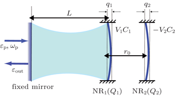
2. Model and solution

As sketched in Fig. 1 , our system consists of a high-quality Fabry–Pérot cavity containing a fixed mirror and a movable mirror NMO 1 . NMO 1 is charged by the bias gate voltage V 1 and subject to the Coulomb force due to another charged NMO 2 with the bias gate voltage − V 2 . The optomechanical cavity of the length L is driven by one strong pump field ɛ p from the left side of the cavity. The output field is represented by ɛ out , q 1 and q 2 represent the small displacements of NMO 1 and NMO 2 from their equilibrium positions, with r 0 the equilibrium distance between the two NMOs. Then, the Hamiltonian in the rotating frame at frequency of the pump field ω p can be given by

where the first term is for the single-mode cavity field with frequency ω c and annihilation (creation) operator c ( c ), and Δ c = ω c ω p is the detuning of the pump field from the bare cavity. The second (third) term describes the vibration of the charged NMO 1 (NMO 2 ) with frequency ω 1 ( ω 2 ), effective mass m 1 ( m 2 ), position operator q 1 ( q 2 ) and momentum operator p 1 ( p 2 ). [ 43 ] The fourth term describes the coupling between NMO 1 and the cavity field with the coupling strength , where L is the cavity length. The fifth term presents the Coulomb coupling between the charged NMO 1 and NMO 2 with the Coulomb coupling strength , [ 41 , 42 ] where the NMO 1 and NMO 2 take the charges Q 1 = C 1 V 1 and Q 2 = − C 2 V 2 , with C 1 ( C 2 ) and V 1 (− V 2 ) being the capacitance and the voltage of the bias gate, respectively. The last term in Eq. ( 1 ) describes the interactions between the cavity field with the input field. The strong pump field possesses the frequency ω p and the amplitude , where P is the power of the pump field and κ is the cavity decay rate.

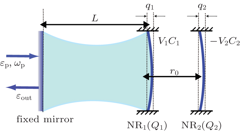
Fig. 1. Schematic diagram of the system.

Considering photon losses from the cavity and the Brownian noise from the environment, we may describe the dynamics of the system governed by Eq. ( 1 ) using the following nonlinear quantum Langevin equations: [ 43 ]

where γ 1 ( γ 2 ) is the decay rate for NMO 1 (NMO 2 ). The quantum Brownian noise ξ 1 ( ξ 2 ) comes from the coupling between NMO 1 (NMO 2 ) and its own environment with correlation function [ 44 ]

where = [exp( ħω m / k B T ) − 1] −1 is the mean number of thermal excitation with k B being the Boltzmann constant, c in is the input vacuum noise operator with nonzero correlation function [ 44 ]

From the Langevin equations above, we can obtain the steady-state mean-values as

where Δ = Δ c gq 1s is the effective cavity detuning.

We can rewrite each Heisenberg operator as its steady-state mean-value plus an additional fluctuation operator with zero-mean value, c = c s + δc , q i = q i s + δq i , p i = p i s + δp i ( i = 1,2). For generating optomechanical entanglement the input power is usually very large, which means | c s | ≫ 1, so we can ignore some small quantity and get the linearized Langevin equations

where G = gc s is the effective coupling strength.

3. Entanglement

In this section, we study the NMO–NMO entanglement and analyze how the degree of entanglement depends on the Coulomb interaction and the frequencies of the two charged NMOs. We also investigate the robustness of the entanglement against temperature.

In order to investigate the optomechanical entanglement, it is more convenient to use the quadratures operators defined by and , and the corresponding Hermitian input noise operators and . Then equation ( 2 ) can be rewritten as the matrix form

in which the transposes of the column vectors u ( t ) and n ( t ) can be expressed as

and the matrix A is

where the effective optomechanical coupling . When the system is stable, it reaches a unique steady state, independently of the initial condition. Since the quantum noises ξ 1(2) and c in are zero-mean quantum Gaussian noises and the dynamics is linearized, the quantum steady state for the fluctuations is a zero-mean bipartite Gaussian state.

The solution of Eq. ( 3 ) can be expressed as

where M ( t ) = exp( A t ). The system is stable only if the real parts of all the eigenvalues of matrix A are negative, which can be derived by applying the Routh–Hurwitz criterion. [ 45 ] We will choose the parameters so that the system is subsequently in a steady state. We define V i j = 〈 u i (∞) u j (∞) + u j (∞) u i (∞)〉/2, which is a 6 × 6 correlation matrix (CM). [ 46 48 ] Here, u T (∞) = (δ q 1 (∞), δ p 1 (∞), δ q 2 (∞), δ p 2 (∞), δ X (∞), δ Y (∞)) is the vector of the fluctuations operators at the steady state. When the system is stable ( t → ∞), we obtain

where Φ kl ( t t ′) = (〈 n k ( t ) n l ( t ′) + n l ( t ′) n k ( t )〉)/2 is the steady-state noise CM. When the stability conditions are satisfied, the steady-state CM satisfies a Lyapunov equation

where D = diag[0, γ 1 (2 1 + 1),0, γ 2 (2 2 + 1), κ , κ ] and j = [exp( ħω j / k B T ) − 1] −1 ( j = 1,2) is the mean thermal excitation number. We can straightforwardly have the solution of the CM with Eq. ( 7 ). However, the explicit expression is too complicated and will not be reported here.

Now, we examine the NMO–NMO entanglement of this optomechanical system. For this purpose, we consider the entanglement of the bipartite subsystems that can be traced over the remaining degrees of freedom. This bipartite entanglement will be quantified by using the logarithmic negativity

where is the lowest symplectic eigenvalue of the partial transpose of the 4 × 4 CM, V bp , associated with the selected bipartition, obtained by disregarding the rows and columns of the uninteresting mode,

and Σ ( V bp ) ≡ det B + det B ′ − 2det C .

For simplicity, we choose all the parameters of the two charged NMOs to be the same, i.e., ω 1 = ω 2 = ω m , γ 1 = γ 2 = γ m . In order to obtain a significant amount of entanglement, we have made a careful analysis in a wide parameter range and found the system parameters, as shown in Table 1 , which are very close to that of performed optomechanical experiments. [ 49 , 50 ] We numerically display the entanglement of the two movable mirrors in Figs. 2 4 .

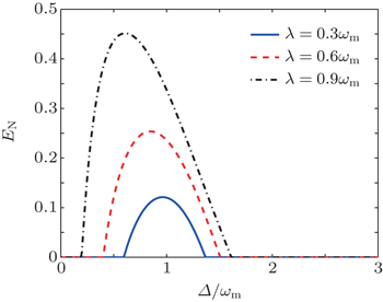
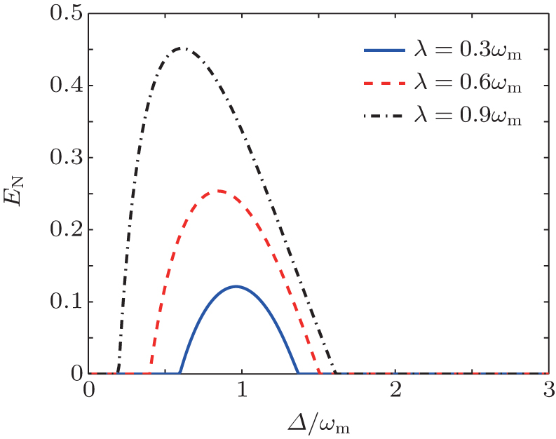
Fig. 2. Plot of the logarithmic negativity as a function of the normalized detuning Δ / ω m .
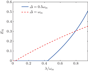
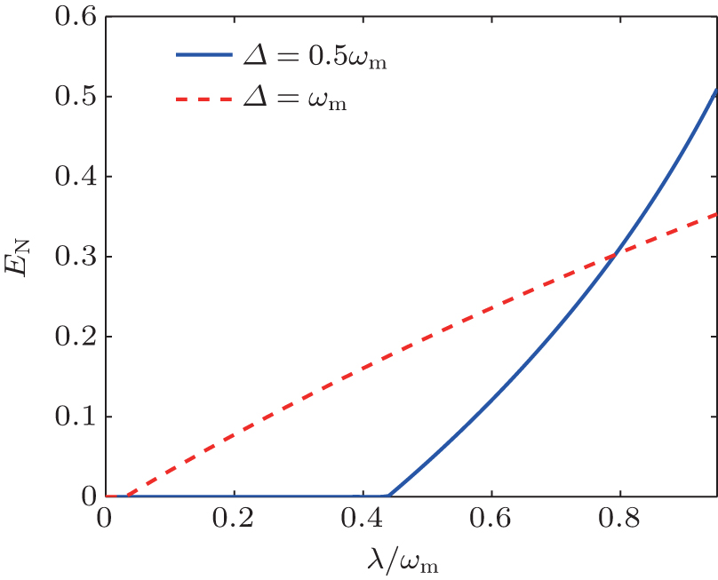
Fig. 3. Plot of the logarithmic negativity as a function of the NMO–NMO coupling strength λ / ω m .
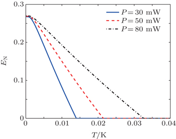
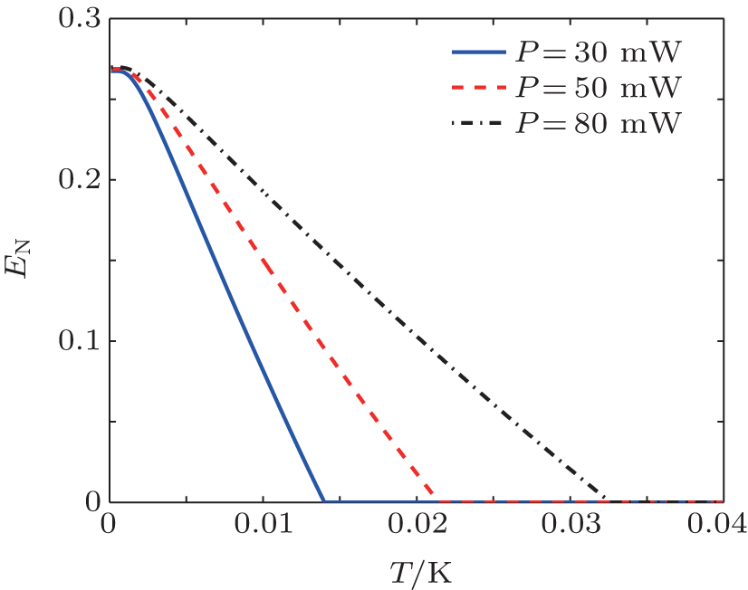
Fig. 4. Plot of the logarithmic negativity versus the environment temperature.
Table 1.

The parameters used in our numerical calculations which are based on the experiment conditions. [ 49 , 50 ]

.

In Fig. 2 , we plot the logarithmic negativity E N versus the normalized detuning Δ / ω m at temperature T = 4 mK and driving power P = 50 mW for three values of the Coulomb coupling strength λ = 0.3 ω m (solid line), λ = 0.5 ω m (dashed line), and λ = 0.9 ω m (dashed-dotted line). It can be clearly seen that the NMO–NMO entanglement is enhanced with the increase of the coupling parameter λ . In the case of λ = 0.3 ω m , the optimal entanglement remains near Δ / ω m = 1 and for λ = 0.9 ω m it is shifted towards lower detuning value around Δ / ω m = 0.5. More importantly, with increasing the NMO–NMO coupling, the range of the entanglement between the two NMOs can be broadened, i.e., from Δ / ω m ∈ [0.6,1.4] (solid line) to Δ / ω m ∈ [0.2,1.6] (dashed-dotted line). The broader the effective detuning, the more easily it is realized in experiments. From Fig. 2 , we can find that the main reason for formation of entanglement between the two nanomechanical oscillators is the existence of Coulomb coupling. The numerical results also show that it is not possible to entangle the two NMOs if there is not the Coulomb coupling.

To further explore the effect of NMO–NMO coupling strength on the entanglement of the two charged NMOs, we plot in Fig. 3 the logarithmic negativity E N versus λ / ω m at temperature T = 4 mK and driving power P = 50 mW. It is obvious that the two oscillators are unentangled below a critical coupling strength λ c and the NMO–NMO entanglement increases nearly linearly with λ in the range λ ∈ [ λ c ,0.95 ω m ]. We find the critical coupling strength λ c1 = 0.03 ω m for the case of Δ = ω m (dashed line), and λ c2 = 0.43 ω m for Δ = 0.5 ω m (solid line). More interestingly, the increase rate in the case of Δ = ω m is smaller than that in the case of Δ = 0.5 ω m .

Figure 4 shows the robustness of the entanglement against the environmental temperature with fixed Coulomb coupling strength λ = 0.6 ω m and detuning Δ = ω m while varying the power of the driving laser. We find that the robustness of NMO–NMO entanglement with respect to the environment temperature is enhanced when we increase the laser power.

In practice, it is hard to achieve two identical NMOs in experiments. For this reason, we plot in Fig. 5 the numerical simulation of the NMO–NMO entanglement when the two charged NMOs have different frequencies ( ω 1 ω 2 ), where we set T = 4 mK, P = 50 mW, and λ = 0.6 ω m . In order to make a comparison, we also plot E N when ω 1 = ω 2 (solid curve). This figure shows that the maximal entanglement between the two charged NMOs is obtained when the frequency of NMO 2 is smaller than the frequency of NMO 1 , i.e., ω 2 = 0.8 ω 1 (dash-dotted curve). When ω 2 = 1.2 ω 1 , the maximal entanglement is decreased and the optimal entanglement is shifted towards higher detuning value (dashed curve). The above discussion implies that we can control the value of NMO–NMO entanglement and the optimal entanglement occurrence through adjusting the Coulomb interaction and frequencies of the two charged NMOs.

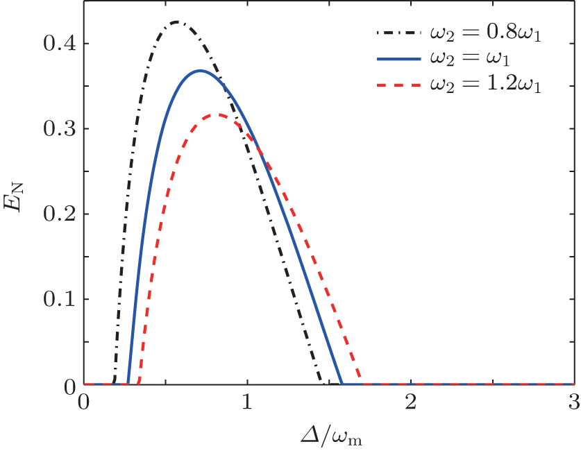
Fig. 5. Plot of the logarithmic negativity as a function of the normalized detuning Δ / ω m when the frequencies of two oscillators are different.
4. Conclusion

In conclusion, we have analyzed the NMO–NMO entanglement in an optomechanical system with two charged NMOs. We show that due to the Coulomb interaction between the two NMOs, they can be entangled. We also find that the generated entanglement can be controlled by adjusting the Coulomb coupling strength and the frequencies of the two charged NMOs: i) The entanglement between the two charged NMOs is enhanced with increasing the Coulomb coupling strength λ . ii) The degree of NMO–NMO entanglement is increased when the frequency of NMO 2 is smaller than the frequency of NMO 1 ( ω 2 > ω 1 ), and is decreased when ω 2 < ω 1 . iii) The points for the optimal entanglement will be shifted to the left for ω 2 < ω 1 and to the right for ω 2 > ω 1 . Besides, we show that increasing the driving power leads to much more robust entanglement against temperature.

Reference
1 Kippenberg T J Vahala K J 2008 Science 321 1172
2 Marquardt F Girvin S M 2009 Physics 2 40
3 Verlot P Tavernarakis A Briant T Cohadon P F Heidmann A 2010 Phys. Rev. Lett. 104 133602
4 Mahajan S Kumar T Bhattacherjee A B ManMohan 2013 Phys. Rev. A 87 013621
5 Huang S Agarwal G S 2011 Phys. Rev. A 83 043826
6 Han Y Cheng J Zhou L 2011 J. Phys. B: At. Mol. Opt. Phys. 44 165505
7 Ma Y H Zhou L 2013 Chin. Phys. B 22 024204
8 Karuza M Biancofiore C Bawaj M Molinelli C Galassi M Natali R Tombesi P Diuseppe G Vitali D 2013 Phys. Rev. A 88 013804
9 Shu J 2011 Chin. Phys. Lett. 28 104203
10 Yan X B Yang L Tian X D et al. 2014 Acta Phys. Sin. 63 204201 (in Chinese)
11 Yan X B Gu K H Fu C B et al. 2014 Chin. Phys. B 23 114201
12 Rocheleau T Ndukum T Machlin C Hertzberg J Clerk A Schwab K 2010 Nature 463 72
13 Miao H Danilishin S Müller-Ebhardt H Chen Y 2010 New J. Phys. 12 083032
14 Vitali D Gigan S Ferreira A Böhm H R Tombesi P Guerreiro A Vedral V Zeilinger A Aspelmeyer M 2007 Phys. Rev. Lett. 98 030405
15 Genes C Mari A Tombesi P Vitali D 2008 Phys. Rev. A 78 032316
16 Akram U Munro W Nemoto K Milburn G J 2012 Phys. Rev. A 86 042306
17 Mi X W Bai J X Song K H 2013 Eur. Phys. J. D 67 115
18 Palomaki T A Teufel J D Simmonds R W Lehnert K W 2013 Science 342 710
19 Joshi C Akram U Milburn G J 2014 New J. Phys. 16 023009
20 Liao J Q Wu Q Q Nori F 2014 Phys. Rev. A 89 014302
21 Ghobadi R Kumar S Pepper B Bouwmeester D Lvovsky A I Simon C 2014 Phys. Rev. Lett. 112 080503
22 Ge W C Al-Amri M Nha H Zubairy M S 2013 Phys. Rev. A 88 022338
23 Zheng Q Zhang D 2013 Chin. Phys. Lett. 30 024213
24 Woolley M J Doherty A C Milburn G J Schwab K C 2008 Phys. Rev. A 78 062303
25 Sete E A Eleuch H 2012 Phys. Rev. A 85 043824
26 Asjad M Agarwal G S Kim M S Tombesi P Di Giuseppe G Vitali D 2014 Phys. Rev. A 89 023849
27 Pinard M Dantan A Vitali D Arcizet O Briant T Heidmann A 2005 Europhys. Lett. 72 747
28 Zhang J Peng K Braunstein S L 2003 Phys. Rev. A 68 013808
29 Huang S Agarwal G S 2009 New J. Phys. 11 103044
30 Tan H Buchmann L F Seok H Li G 2013 Phys. Rev. A 87 022318
31 Børkje K Nunnenkamp A Girvin S M 2011 Phys. Rev. Lett. 107 123601
32 Woolley M J Clerk A A 2013 Phys. Rev. A 87 063846
33 Mancini S Vitali D Tombesi P 2003 Phys. Rev. Lett. 90 137901
34 Pirandola S Mancini S Vitali D Tombesi P 2003 Phys. Rev. A 68 062317
35 Pirandola S Mancini S Vitali D Tombesi P 2004 J. Mod. Opt. 51 901
36 Pirandola S Vitali D Tombesi P Lloyd S 2006 Phys. Rev. Lett. 97 150403
37 Zhou L Han Y Jing J T Zhang W P 2011 Phys. Rev. A 83 052117
38 Hartmann M J Plenio M B 2008 Phys. Rev. Lett. 101 200503
39 Löw U Emery V J Fabricius K 1994 Phys. Rev. Lett. 72 1918
40 Bohm D Pines D 1953 Phys. Rev. 92 609
41 Ma P C Zhang J Q Xiao Y Feng M Zhang Z M 2014 Phys. Rev. A 90 043825
42 Hensinger W K Utami D W Goan H S Schwab K Monroe C Milburn G J 2005 Phys. Rev. A 72 041405(R)
43 Agarwal G S Huang M 2012 Phys. Rev. A 85 021801(R)
44 Genes C Vitali D Tombei D Gigan S Aspelmeyer M 2008 Phys. Rev. A 77 033804
45 DeJesus E X Kaufman C 1987 Phys. Rev. A 35 5288
46 Adesso G Illuminati F 2007 J. Phys. A 40 7821
47 Weedbrook C Pirandola S Garcia-Patrón R Cerf N J Ralph T C Shapiro J H Lloyd S 2012 Rev. Mod. Phys. 84 621
48 Olivares S 2012 Eur. Phys. J. Special Topics 203 3
49 Schliesser A Riviere R Anetsberger G Arcizet O Kippenberg T J 2008 Nat. Phys. 4 415
50 Gigan S Böhm H R Paternostro M Blaser F Langer G Hertzberg J B Schwab K C Bäuerle D Aspelmeyer M Zeilinger A 2006 Nature 444 67