To study the phase equilibrium and ground-state structures of the Cd _{1– x} Zn _x S alloys, it is necessary to compute the total energies of all possible configurations by placing Cd and Zn atoms on N sites of the Bravais lattice. It is almost impossible to obtain the total energies of all possible configurations exhaustively by first-principles, because the number of possible configurations 2 ^N is enormous. The cluster expansion (CE) method constructs an Ising-like Hamiltonian for calculating the energies of different atomic configurations. This method has been illustrated in Refs. [ 34 ]–[ 38 ] in detail. For Cd _{1– x} Zn _x S alloys, each configuration is described by a set of “spin” occupation variables σ _i at i sites of the lattice, and σ _i = +1 or –1 depending on which kind of atoms occupied site i .

The CE parameterizes the configurational energy (per exchangeable cation) as a polynomial in “spin” occupation variables

We introduced the cross-validation (CV) score as the criterion to evaluate the predictive power of the cluster expansion. The CV score is defined as

The electronic-structure total-energy calculations of ordered structures, which are required for the construction of the cluster expansion Hamiltonian, were performed using the Vienna ab initio simulation package (VASP). ^{[ 42 , 43 ]} The interaction between the core and the valence electrons was included by the frozen-core projector augmented wave (PAW) method. ^{[ 44 , 45 ]} The valence electron configurations for the pseudopotentials are Cd: 4d ¹⁰ 5s ² , Zn: 3d ¹⁰ 4s ² , and S: 3s ² 3p ⁴ . Both lattice parameters and ionic positions were fully relaxed for all supercells. The plane-wave energy cutoff was 370 eV. The generalized gradient approximation (GGA) functional of Perdew–Burke–Ernzerhof (PBE) was introduced to describe the exchange–correlation energy. ^{[ 46 ]} ATAT was used as a script interface to VASP. This script defines a parameter called KPPRA, which automatically sets up the k -point mesh for similar systems. In this work, KPPRA was set to 2000, which for the primitive cells of cubic and hexagonal structures translates to 7×7×7 and 9×9×5 k -point grids, respectively. The convergence tests showed that the increases of energy cutoff and k -points change the total energy by less than 0.01 meV.

We adopted the conventional Monte Carlo simulations to obtain the phase diagrams of the WZ and the ZB Cd _{1– x} Zn _x S alloys as well as the spatial distributions of Cd and Zn atoms in the two structures of Cd _0.5 Zn _0.5 S alloys. We calculated their two-phase equilibrium states. In this paper, we adopted 20×20×20 and 30×30×16 supercells to calculate the phase diagrams for the WZ and the ZB Cd _{1– x} Zn _x S alloys, respectively. The average time for the given precision on the average concentration of the alloy was set to 0.1% in the current simulations. A detailed description of the algorithm underlying this program can be found in Ref. [ 40 ]. The energy of the system was specified by the cluster expansion Hamiltonian. The spatial distributions of Cd and Zn atoms in Cd _{1– x} Zn _x S alloys were also studied. To make the simulation feasible, we kept Cd and Zn atoms fixed at their respective lattice sites and ignore other defects.

In the cluster expansions of the WZ and the ZB Cd _{1– x} Zn _x S alloys, 68 and 57 input structures have been used, and the CV scores are 1.3 meV and 2.3 meV, respectively. The small CV scores indicate that the predictive ability of the cluster expansions is excellent in this work. The ECIs of the WZ and the ZB Cd _{1– x} Zn _x S alloys obtained from the cluster expansion are given in Table 1 , and are also shown in Fig.  1 . In Table  1 , we adopt J (0, 1), J (1, 1), J (2, 1,…, m ), and J (3, 1,…, m ) to represent the empty, point, pair, and three-body clusters, respectively. Coordinates are in a fraction of lattice vectors. The cluster size is defined as the length of the longest pair contained in the cluster.

Fig. 1.

	Figure Option View Download New Window
	Fig. 1. ECIs of WZ and ZB Cd 1– x Zn x S alloys versus cluster diameter. The horizontal axis represents the cluster diameters; the first is for pair clusters, and the next is for triplet clusters. The cluster diameter is defined as the length of the longest pair contained in the cluster.

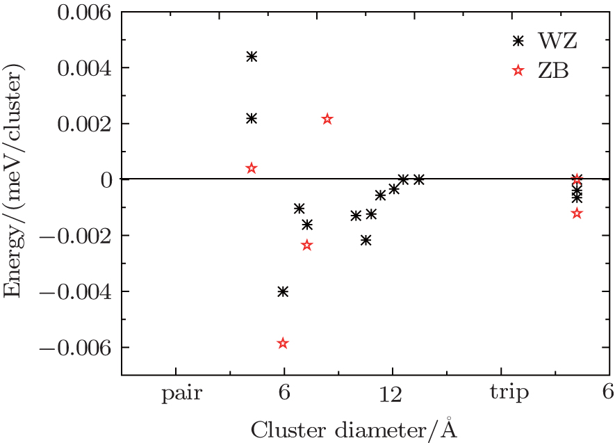
Table 1.

Table 1.

Table 1. ECIs of the wurtzite and zinc-blende Cd 1– x Zn x S alloys. . Phase Cluster Coordinates Size/Å Multiplicity ECI WZ J (0,1) 1 0.06875 J (1,1) (0.333,0.667,0.003) 2 0.00214 J (2,1) (0.667,0.333,0.503) (0.333,–0.333,1.003) 4.184 6 0.00219 J (2,2) (0.667,0.333,0.503) (–0.333,–0.667,0.503) 4.196 6 0.00440 J (2,3) (0.333,0.667,0.003) (–0.333,–0.667,–0.497) 5.925 6 –0.00401 J (2,4) (0.667,0.333,0.503) (-0.333,-0.667,-0.497) 6.822 2 –0.00105 J (2,5) (0.333,0.667,0.003) (1.667,2.333,–0.497) 7.268 6 -0.00161 J (2,6) (0.667,0.333,0.503) (–0.333,-1.667,1.503) 9.968 6 –0.00129 J (2,7) (0.333,0.667,0.003) (0.667,1.333,–1.497) 10.516 6 –0.00217 J (2,8) (0.333,0.667,0.003) (–1.667,–1.333,–0.997) 10.815 12 -0.00123 J (2,9) (0.333,0.667,0.003) (–0.333,–1.667,–1.497) 11.322 6 –0.00056 J (2,10) (0.667,0.333,0.503) (-0.667,-1.333,2.003) 12.075 12 –0.00033 J (2,11) (0.333,0.667,0.003) (–2.333,-2.667,0.503) 12.584 6 0.00000 J (2,12) (0.333,0.667,0.003) (–1.333,–1.667,–1.497) 13.454 12 0.00000 J (3,1) (0.667,0.333,0.503) (0.333,–0.333,1.003) (–0.333,-0.667,0.503) 4.196 6 -0.00065 J (3,2) (0.667,0.333,0.503) (0.333,–0.333,0.003) (–0.333,-0.667,0.503) 4.196 6 –0.00038 J (3,3) (0.667,0.333,0.503) (–0.333,0.333,0.503) (–0.333,–0.667,0.503) 4.196 2 0.00000 ZB J (0,1) 1 0.12673 J (1,1) (1.00,1.00,1.00) 4 0.00424 J (2,1) (1.00,0.50,0.50) (1.50,0.50,0.00) 4.191 24 0.00040 J (2,2) (0.50,0.50,1.00) (1.50,0.50,1.00) 5.927 12 –0.00586 J (2,3) (0.50,0.50,1.00) (1.50,1.00,1.50) 7.259 48 –0.00235 J (2,4) (0.50,0.50,1.00) (1.50,0.50,0.00) 8.382 24 0.00216 J (3,1) (1.00,0.50,0.50) (1.50,0.50,0.00) (1.00,0.00,0.00) 4.191 16 -0.00122 J (3,2) (1.00,0.50,0.50) (0.50,0.50,0.00) (1.00,0.00,0.00) 4.191 16 0.00000

Table 1. ECIs of the wurtzite and zinc-blende Cd 1– x Zn x S alloys. .

As we can see in Table  1 , the cluster expansion of the WZ Cd _{1– x} Zn _x S alloys includes interactions up to twelve neighboring pairs and three three-body terms to obtain the desired CV score. For the ZB Cd _{1– x} Zn _x S alloys, it includes interactions of four neighboring pairs and two three-body terms to obtain the desired CV score. The presence of the three-body terms implies an asymmetric miscibility gap in the Cd _{1– x} Zn _x S system. ^{[ 47 ]} It is evident that the first and the second neighboring pair ECIs for WZ and the first neighboring pair ECIs for ZB are positive, which is related to the ordering tendency of Cd _{1– x} Zn _x S. However, the third and the fourth neighboring pair ECIs for WZ as well as the second and the third neighboring pair ECIs for ZB are negative, which appears to counteract with the ordering tendency and is related to the tendency of phase separation. ^{[ 48 , 49 ]} As shown in Fig.  1 , the magnitude of ECI is reduced gradually as the distance and the cluster size increase, and the convergence is obtained ultimately.

The formation energies of WZ and ZB Cd _{1– x} Zn _x S solid solutions are shown in Figs.  2(a) and 2(b) , respectively. The formation energy Δ E _f ( σ ) of configuration σ is calculated as follows:

Fig. 2.

Figure Option View Download New Window

Fig. 2. Cluster expansion of formation energies and direct enumeration ground-state search results of Cd 1– x Zn x S solid solutions: (a) WZ structure, (b) ZB structure. The “known stru." denotes structures whose energies have been calculated from first-principles. The “known gs” indicates the ground states that have been confirmed by first-principles calculations. The “predicted” denotes structures whose energies have been predicted from the cluster expansion and ab initio energies are known.

We computed the amount of charge transfer between cations and anions in each input structure of WZ and ZB Cd _{1– x} Zn _x S alloys by Bader charge analysis technique. ^{[ 53 – 55 ]} We obtained the average amount of charge transfer to S atoms for each Zn concentration. The statistical error of the average charge transfer was too large for some concentrations with a small number of structures (less than 3), so we did not take them into consideration. As the electrons of Cd and Zn atoms transfer to S atoms in WZ and ZB Cd _{1– x} Zn _x S alloys, the amount of charge gained by S atoms shows the ionicity of these alloys. As we can see in Fig.  3 , the average amount of charge gained by S atoms in WZ Cd _{1– x} Zn _x S alloys is higher than that in ZB Cd _{1– x} Zn _x S alloys except when x is 0 and 1. It indicates that the ionicity of WZ Cd _{1– x} Zn _x S is stronger than that of ZB Cd _{1– x} Zn _x S. The average amount of charge gained by S atoms increases with the increase of the Zn concentration in the two structures. It means that the ionicity of Cd _{1– x} Zn _x S alloys is stronger with the doping of Zn.

Fig. 3.

	Figure Option View Download New Window
	Fig. 3. The average amount of charge transfer to S atoms versus the Zn concentration in WZ and ZB Cd 1– x Zn x S alloys.

Figure  4 shows the calculated phase diagrams of WZ and ZB Cd _{1– x} Zn _x S alloys. In Fig.  4 , the binodal curves correspond to the coexistence of CdS and ZnS phases. Inside the curves, the phase separation can occur thermodynamically for both the WZ and the ZB Cd _{1– x} Zn _x S alloys. Outside the curves, the Cd _{1– x} Zn _x S solid solutions are stable and homogenous. As shown in Fig.  4 , for the WZ and the ZB Cd _{1– x} Zn _x S alloys, the consolute temperatures are 655 K and 604 K, respectively, and the corresponding consolute concentrations are 0.646 and 0.695. Both binodal curves are asymmetric. The binodal curve of WZ Cd _{1– x} Zn _x S we obtained is close to that of Lu et al. ^{[ 24 ]} Their result shows that the consolute temperature of WZ Cd _{1– x} Zn _x S is 613 K, which is just 42 K lower than ours. The consolute concentration they obtained is about 0.68, and is in fair agreement with our result. It should be noted that the computational method we adopted is different from that of Lu et al. ^{[ 24 ]} though the results are similar. Zhang et al. ^{[ 12 ]} found that at the temperature of 723 K, the WZ Cd _{1– x} Zn _x S solid solution can be synthesized uninterruptedly and homogenously. While at 673 K, the Cd _{1– x} Zn _x S film is rough and uneven; its surface appears to exhibit the phenomenon of segregation, which is consistent with the consolute temperature of 655 K obtained by us. All of these indicate that the phase diagram of the WZ Cd _{1– x} Zn _x S alloy we obtained is reliable. We have also computed the phase diagram of the ZB Cd _{1– x} Zn _x S solid solutions by the same method. The calculated consolute temperature T _c of the ZB Cd _{1– x} Zn _x S solid solutions is 604 K, which is much lower than 1278 K obtained by Zhou et al. ^{[ 25 ]} Our results agree well with the experiment, as the synthesis was carried out at 513 K ( x = 0.13 and 0.66). ^{[ 56 , 57 ]}

Fig. 4.

	Figure Option View Download New Window
	Fig. 4. Phase diagrams of WZ and ZB Cd 1– x Zn x S alloys.

We calculated the spatial distributions of Cd and Zn (active atoms) in WZ and ZB Cd _0.5 Zn _0.5 S alloys at the temperatures of 300 K, 600 K, 650 K, 700 K and 300 K, 550 K, 600 K, 650 K, respectively. As we can see in Fig.  5 , there is a phase separation in the WZ Cd _0.5 Zn _0.5 S alloy at the temperatures of 300 K and 600 K, which means that the coexistence of CdS and ZnS phases is stable at low temperature. As the temperature increases, the alloy tends to be homogeneous, especially when the temperature is over 650 K. The ZB Cd _0.5 Zn _0.5 S solid solution has a similar tendency as the temperature increases.

Fig. 5.

	Figure Option View Download New Window
	Fig. 5. Snapshots of (a)–(d) WZ and (e)–(h) ZB Cd 0.5 Zn 0.5 S alloys at different temperatures. Red and blue spheres represent Zn and Cd atoms, respectively.

In order to study the spatial distributions of Cd and Zn atoms in WZ and ZB Cd _0.5 Zn _0.5 S alloys at different temperatures quantitatively, we divided the WZ and the ZB supercells into 1800 and 2000 segments, respectively. Each segment has 16 active atoms for both WZ and ZB Cd _0.5 Zn _0.5 S alloys. We counted the number of Cd atoms in each segment. The standard deviation σ was computed as follows:

Fig. 6.

	Figure Option View Download New Window
	Fig. 6. The standard deviation σ of WZ and ZB Cd 0.5 Zn 0.5 S alloys as a function of temperature.