To obtain the structural information of a biological sample, the image should be first taken and digitalized by a camera. Although the electron cryo-microscope has to be operated under a micrometer defocus condition which is not optimal for performance, most modern TEMs equipped with a field emission gun are still able to deliver structural information better than 2 Å resolution to the camera plane. Therefore, camera performance is critical for the obtainable resolution of the next 3D reconstruction step.

There are at least three types of image recording media or cameras that are used for CryoEM, i.e., film, charge-coupled device (CCD) camera and complementary metal-oxide semiconductor (CMOS) camera. There is also another image recording medium, the electronic image plate, which is mostly used to record electron diffraction and is seldom used in CryoEM and will not be discussed here. Both film and cameras first convert the incident electrons to detectable light signal by a phosphor scintillator layer, and then record the light intensity by either a scanner or an electronic detector. During the conversion and recoding step, the input signal might be attenuated and extra noise might be added. ^{[ 7 – 9 ]} To characterize the performance of an image recording system, the detective quantum efficiency (DQE) and modulation transfer function (MTF) have been widely adopted. Because of combining the influences from most of the performance-related factors, including MTF (discussed later), DQE is thought to be a comprehensive indictor of camera performance. DQE describes the squared ratio of the output and the input SNR at different spatial frequencies in Fourier space. ^{[ 10 , 11 ]} The DQE of traditional cameras usually decays rapidly as the spatial frequency increases, typically from ∼ 0.4 at low frequency to ∼ 0.2 or worse at high frequency. ^{[ 11 ]} For a digital image, the maximum spatial frequency in the Fourier transform of the image is half of the reciprocal of the image pixel size, termed Nyquist frequency. In material science, the sample is usually imaged at high magnification, which corresponds to an over-sampled small pixel size and wide spatial frequency range. All use-ful signals in Fourier transform of the image, typically within ∼ 1 Å ^{− 1} range, are located in the low-frequency region of the camera, where the camera has the best performance. Together with the high dose and corresponding high SNR, the decay of ∼ 0.4 is a very subtle influence on the image analysis. However, for a biological sample, much lower magnification has to be used to cover sufficient imaging area in order to increase the efficiency of data collection or cover a large enough cellular area within a single image. The low magnification leads to a large pixel size and, accordingly, a spatial frequency range covering most of the spatial frequency space of the camera. Consequently, camera performance at high frequency is very critical.

The low-frequency signal contributes to image contrast which is important to recognize the biological sample embedded in vitrified ice and to guide the 3D alignment. The highfrequency signal contains high-resolution details, for example, the side chain of the amino acid and ligand bound to the protein. Under the low-dose imaging condition, the input SNR of a biological sample is often less than 0.1. The additional signal decay and noise from the camera, especially at high resolution, smear out the high-resolution structural information to undetectable level. For this reason, the low performance of traditional cameras already makes the atomic resolution impossible before the subsequent image-processing step.

A biological sample must be stabilized at the angstrom level to obtain nanometer or atomic resolution. There are at least two types of sources of instability. The first is mechanical motion or vibration. Unstable specimen stage, temperature gradient between the biological sample holder cooled by liquid-nitrogen and the microscope at room temperature, as well as environmental vibrations cause sample drift. The second source is the so-called beam-induced motion. ^{[ 12 ]} When the high-energy electron beam hits the biological sample and stimulates the escape of secondary electrons, the surface of the insulated biological sample will be charged (Fig.  1 ). ^{[ 13 ]} These charges gradually accumulate and might immigrate along the surface, refracting the electron beam and resulting in image drift. This beam-induced drift is usually uneven within the imaging area. Meantime, the energy from the electron beam can also be absorbed by the sample and cause the thin ice layer to bend. The absorbed energy can also cause small thermal motion of the water molecules in amorphous ice, termed Brownian motion, which might further displace the embedded protein molecules. ^{[ 14 , 15 ]} Consequently, in addition to drifting, the biological samples might be slightly tilted or rotated with the bent ice layer. ^{[ 12 ]} Together, a sample illuminated by an electron beam usually has uneven and complicated behaviors, including drift, tilt and rotation. These combined effects of mechanical and beam-induced instability make the image blurred. Empirically, more than 90% of images in a dataset with hundreds of images could be significantly influenced by the blurring, and show smeared Thon rings along the direction of motion.

Due to the low SNR and the requirement for orientation coverage in single-particle CryoEM, thousands or even millions of images are merged to obtain the 3D reconstruction of a target sample. Although these images are taken from different molecules, it is assumed that all molecules have the same conformation. The heterogeneous or flexible region in molecules will be averaged out and will disappear in the final reconstruction. Even more seriously, the heterogeneity can cause the failure in determining 3D orientation parameters against the same 3D reference, and lead to overall low resolution or even wrong results.

Heterogeneity in conformation or composition is usually a natural property of biological macromolecules and coherent with its biological function. For the x-ray crystallographic approach, heterogeneity must be carefully removed through a series of biochemistry modifications, such as mutations and truncations, before a successful crystallization. Without the need for crystallization, CryoEM has a slightly higher tolerance for sample heterogeneity, if the heterogeneity is limited to a small region of a large molecule. However, in practice the requirement for overall homogeneity is almost as critical as that for the crystallographic approach. Stabilizing and isolating homogenous molecules are always necessary to reach atomic resolution by single-particle CryoEM.

In the past five years, a new type of camera, named direct detection detector (DDD) camera, was developed and commercially available. The DDD camera has a much higher DQE than traditional cameras, and provides improved contrast and SNR at high resolution. ^{[ 16 , 23 – 26 ]} Such improvements make the structure determination of small molecules and atomic resolution more reachable than ever. Currently, there are three commercially available DDD cameras, i.e., the DE series camera (Direct Electron Company, San Diego, CA, USA), Falcon camera (FEI Company, Hillsboro, OR, USA), and K2 Summit camera (Gatan Company, Pleasanton, CA, USA). The first two cameras linearly accumulate the signal stimulated by the incident electron (referred to as DDD linear cameras below). In particular, the K2 camera works in a different mode, named electron counting, which recognizes each primary electron and digitally counts the electron inputs (referred to as DDD counting camera below). ^{[ 16 ]} The electron counting technology further improves the DQE on top of the DDD linear camera, and makes the counting camera closer to an ideal pixelated camera.

3.1.2. Counting electrons

The structural information of a biological sample is carried by the electron wave and presented as the number of electrons in different spatial positions, proportional to the probability density function of the beam. Therefore, the ideal image recording is to count the number of electrons striking each pixel. ^{[ 24 ]} For this purpose, the first electron-counting camera (K2 Summit ^TM , Gatan) was developed using a different mechanism from those of traditional and DDD linear cameras. The K2 camera has an intrinsic high frame rate, i.e., 400 frames/sec, enabling each primary electron to be individually recorded. ^{[ 16 , 28 ]} Assisted by high-speed computing, each frame is immediately analyzed to centroid and the incident primary electrons counted within this frame (Fig.  2 ). The high frame rate makes the number of electrons arriving in each frame be so small that they are well separated and distinguishable. The final output image is the sum of these intrinsic frames. The K2 camera can locate electrons with half-pixel position accuracy, which is termed centroiding or super resolution mode, and hence the effective camera size is 2 × 2 larger than its physical size.

Fig. 2.

Figure Option View Download New Window

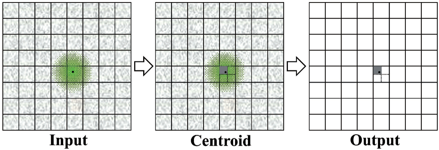Fig. 2. Diagram of counting and centroiding with half-pixel precision. The lattice of squares denotes the pixel matrix of a counting camera, and the noisy background represents the readout noise. The small black dot denotes an incident primary electron which stimulates signals (green spot) around it. The peak position of the green spot is centroided with half-pixel precision, and then its intensity is digitalized and counted as one. Consequently, the point spread effect and readout noise are eliminated from the final output image.

Compared with the DDD linear camera, counting has at least three advantages. ^{[ 28 ]} First, the point spread effect caused by electron striking is totally removed by the counting procedure. Second, the camera is almost free of noise. During counting, only the number of electrons is digitally counted, and all the background noise that appears in the intrinsic frame is discarded. For the DDD linear camera, the remaining pointspread signal together with all background readout noise and Landau noises (from the statistical energy fluctuation when each primary electron strikes the camera) are accumulated. Third, the intensity variation of electron striking is eliminated. The signal stimulated by electron striking is usually different for each electron and varies with incident position. By counting, the intensity of each electron is digitalized to one, hence, the detected intensity differences among electrons are eliminated, while DDD linear camera and traditional cameras simply accumulate all the electron signals and cannot correct this intensity variation. The intensity variation usually contributes to low-frequency noise of the image. ^{[ 29 ]} Therefore, the counting camera has less low-frequency noise than the traditional cameras.

Considering the above advantages, the DQE of the counting camera is significantly improved, that is, much stronger signal at both low- and high-frequency range can be recorded than the accumulation mode of DDD linear cameras (Fig.  3 ). A remarkable feature of counting image is much more visible Thon rings in the power spectrum of frozen hydrated ice images (Fig.  4 ). ^{[ 28 ]} In particular, at low frequency the DQE of the counting camera can be two times better than that of the DDD linear camera, which means the counting camera has better contrast. As shown in Fig.  4(b) , even with a low defocus of ∼ 1.1 μm on a 300 kV electron microscope, the frozen hydrated archaeal 20S proteasome is still clearly visible. This feature enhances the capability of single-particle CryoEM for small molecules.

Fig. 3.

Figure Option View Download New Window

Fig. 3. (a) DQE of three cameras. [ 16 ] Gatan UltranScan Camera (black) is a traditional camera with a scintillator. The accumulation mode (blue) and counting mode (red) of the K2 camera represent the DDD linear camera and counting camera, respectively. Note that centroiding with half-pixel precision doubles the camera size. (b) Rotational average of the power spectrum of two images of Pt/Ir film, respectively taken with the linear accumulation mode (blue) and counting mode (red) of the K2 camera. [ 28 ] The inset figure shows the spectrum SNR (SSNR) calculated from the two curves in the main figure, where the higher red curve (counting mode) confirms the DQE observed in panel (a).

Fig. 4.

	Figure Option View Download New Window
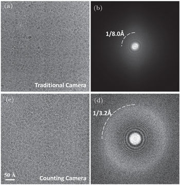
	Fig. 4. (a) An image of a frozen hydrated archaeal 20S proteasome sample taken on a TVIPS F816 traditional CMOS camera with 1.6 μm defocus and 200 kV accelerating voltage, and (b) its power spectrum. Panels (c) and (d) are similar to panels (a) and (b), respectively, but were taken with a K2 summit counting camera with 1.1 μm defocus and 300 kV accelerating voltage.

However, the counting camera must be operated with a relatively weak beam, i.e., using a low dose rate. ^{[ 28 ]} When more than one electron strikes the same position, the counting camera is not able to distinguish them and just simply counts them as one electron. Consequently, the other electrons are undercounted. This effect is called coincident loss, and must be carefully considered during the application. For the K2 counting camera with an intrinsic frame rate of 400 frames/sec, the dose rate of ∼ 10 e/pixel/sec or lower is recommended. The disadvantage of the low dose rate is that a prolonged exposure time must be used, typically 5–20 s. Therefore, the image will be more sensitive to specimen instability than traditional and DDD linear cameras. Fortunately, the motion during a long exposure can be compensated by motion correction technology (discussed below).

A benefit of the DDD camera is its high output frame rate. All commercially available DDD cameras can output up to 40 frames per second, called dose fractionation or movie mode. That is, within one exposure, the DDD camera can sequentially take multiple images (frames) rather than a single image. This feature brings the possibilities of analyzing and correcting imperfections in an image, which was previously impossible.

Motion correction was the first technique that benefited from dose fractionation. As mentioned in the previous section, motion from the specimen instability blurs an image, especially high-frequency (high-resolution) signals (Fig.  5(a) ). This is one of the key barriers to atomic resolution. With dose fractionated frames, the sample movements during exposure are recorded in a movie with multiple frames. If the relative shifts among frames can be determined, the motion is correctable by shifting each frame to the same position followed by summing them together (Figs.  5(b) and 5(c) ). Many approaches have been developed for this purpose, for example, the approach based on cross correlation between two adjacent frames and the refinement approach by comparing any one frame with the sum of all the other frames. We also developed a robust motion correction approach with redundant measurements of the whole frame motion. ^{[ 16 ]} All the possible comparisons between any two frames, which calculates the relative shift between the two compared frames, were carried out. Each comparison is formulated as an equation of an over-determined equation set, in which the number of equations is much more than the number of unknown frame shifts. Solving the over-determined set gives a least-square solution of the frame shifts. This approach improved the resolution of a 3D reconstruction of frozen hydrated archaeal 20S proteasome from 4.2 Å to 3.4 Å. Due to the motion not even being on an image, the further sub-region correction and local motion correction have also been developed to further improve the image quality. ^{[ 16 , 30 ]}

Fig. 5.

	Figure Option View Download New Window
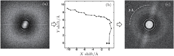
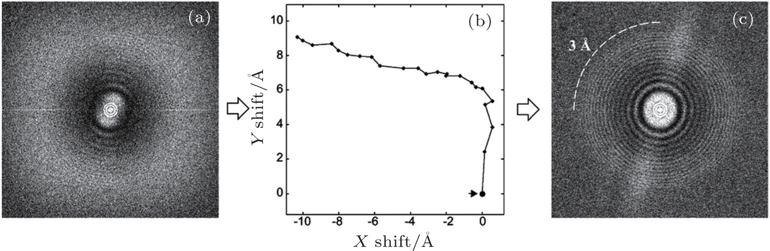	Fig. 5. Thon ring before and after motion correction. [ 16 ] (a) The power spectrum of an image with motion. The Thon ring is smeared by the motion. (b) The trace of motion in panel (a), which is measured using the redundant approach. (c) The power spectrum after motion correction. The smeared Thon ring is recovered to at least 3 Å resolution.

In addition to motion correction, the total dose used for one exposure can now be extended to greater than 60 e/Å ² . Because the dose is divided by many frames, rather than one single image, the dose can be easily selected by summing a part of the frames. Electron radiation rapidly damages the high-frequency signal with the increasing of frame number, but less to the low-frequency signal. Therefore, the advantage of using a high dose is to increase image contrast which is contributed by low-frequency signal. High contrast will help to improve particle picking and 2D/3D alignment. In the final 3D reconstruction, the frames that are severely damaged by the radiation can be removed or low-pass filtered to remove the damaged high-frequency signals. ^{[ 16 , 30 , 31 ]} Such processing has been adopted in the final step of near-atomic resolution 3D reconstruction, and, typically, can gain the resolution with 0.1–0.5 Å.

Sample heterogeneity is always the first thing to be dealt with before obtaining a high-resolution 3D reconstruction by single-particle CryoEM. Besides the biochemistry purification, computational technology provides another way to isolate bio-macromolecules with different conformation or composition, termed classification. The classification can be performed at 2D and 3D levels. For 2D classification, it classifies the 2D images based on their similarities into many classes presumably different in projection direction, conformation or composition. The 2D classification is efficient for particle screening and isolating bad particles, and has been well established. For 3D classification, it is much more challenging than the 2D case due to the complexity of 3D alignment when heterogeneity is present. Owing to the low contrast of CryoEM images, it is very uncertain to recognize a different feature and assign the corresponding image to a certain class. Recently, a maximum-likelihood (ML) based method was developed and implemented with a user-friendly interface. ^{[ 32 ]} Different from the traditional method which assigns each particle image to a specific class, ML method calculates the probability of a particle image belonging to a class. Based on the probability, each particle is assigned and contributes to all classes but with different weighting. The ML method has been proved efficient by a series of high-resolution 3D reconstructions of biological macromolecules with small size and heterogeneity. ^{[ 20 , 21 , 33 , 34 ]}