

Improvements in continuum modeling for biomolecular systems
[Qiao Yu , Lu Ben-Zhuo †,  ]
]
]
|
|


† Corresponding author. E-mail:
Project supported by the National Natural Science Foundation of China (Grant No. 91230106) and the Chinese Academy of Sciences Program for Cross & Cooperative Team of the Science & Technology Innovation.
Modeling of biomolecular systems plays an essential role in understanding biological processes, such as ionic flow across channels, protein modification or interaction, and cell signaling. The continuum model described by the Poisson– Boltzmann (PB)/Poisson–Nernst–Planck (PNP) equations has made great contributions towards simulation of these processes. However, the model has shortcomings in its commonly used form and cannot capture (or cannot accurately capture) some important physical properties of the biological systems. Considerable efforts have been made to improve the continuum model to account for discrete particle interactions and to make progress in numerical methods to provide accurate and efficient simulations. This review will summarize recent main improvements in continuum modeling for biomolecular systems, with focus on the size-modified models, the coupling of the classical density functional theory and the PNP equations, the coupling of polar and nonpolar interactions, and numerical progress.
Modeling of biomolecular systems containing ionic particles and biomolecules is an important approach in life science for investigating the electrostatic properties, such as ion distributions, electrostatic free energy, reactive rate, and ion current. [ 1 – 9 ] Based on a mean field framework, the continuum model treats ions in solution as continuum distributions rather than discrete particles, avoiding large degrees of freedom in computation. In the general case, the Poisson–Nernst– Planck (PNP) equations are utilized for continuum modeling of biomolecular systems. In particular, in the equilibrium state, the ion density is assumed to obey the Boltzmann distribution, and the Poisson–Boltzmann (PB) model can describe the electrostatic interactions in a solvated system. It is noticed that the steady-state PNP equations can be reduced to the PB equation under equilibrium conditions. [ 10 ]
Although the continuum model has wide applications and has achieved great success in predicting many thermodynamic properties, the facts that ions are regarded as point charges and the model does not take into account the ionic volume exclusion and the ion–ion correlations make it unfeasible for systems where these effects are pronounced. [ 11 – 24 ] The continuum model can lead to a high unphysical concentration of counter ions in the vicinity of the biomolecule and miss the phenomena of ionic layering, overcharging or charge inversion, and like-charge attraction. [ 10 , 18 , 25 , 26 ]
In the past few decades, a large number of methods have been developed to improve the continuum model in order to precisely simulate the biomolecular systems and obtain more reasonable computational results. The ionic size effects are incorporated in the continuum model by taking into account the volume exclusion, resulting in a size-modified model. [ 11 – 14 , 16 – 18 ] Combining the classical density functional theory (DFT) with the PNP equations has also been proposed to improve the continuum model through the inclusion of an excess chemical potential, which is the variation of excess Helmholtz free energy with respect to the ion concentrations. [ 20 – 24 , 27 ] Biomolecular exclusion expressed by a characteristic function, as well as other polar and nonpolar interactions, is added to the free energy to obtain optimal volume and surface and minimum free energy. [ 28 – 30 ] Apart from these modifications, some other improvements to account for effects neglected by the traditional continuum models will be briefly discussed.
Along with relevant developments in physics, computer science, and mathematics, numerical methods have also been developed to obtain more accurate and efficient results. [ 1 , 31 ] A new treatment on the boundary is provided to give high solution accuracy and parallelization by using MPI and GPU, and the cilk plus system is used to increase the speed of computations.
The purpose of this review is to provide an overview of the continuum models, their recent improvements, and numerical progress for modeling the biomolecular systems. In Section 2, we discuss the continuum model governed by the PB/PNP equations. The improvements and numerical progress are presented in Section 3 and Section 4, respectively. Finally, we provide the conclusions in Section 5.
In the simulation of solvated biomolecular systems, the computational region Ω is composed of two parts, the biomolecular region Ω m with dielectric constant ɛ m , and the solution region Ω s with dielectric constant ɛ s . Figure
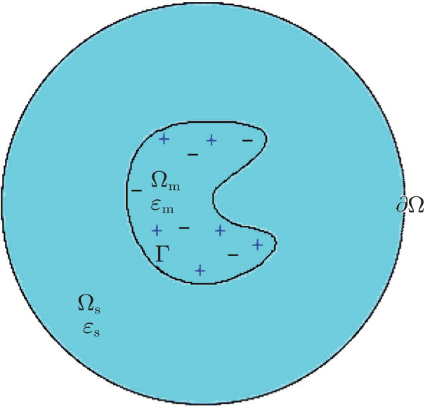 | Fig. 1. Illustration of a solvated biomolecular system. |
The PB equation in Ω takes the form


In the general case, the PNP equations are given as follows:


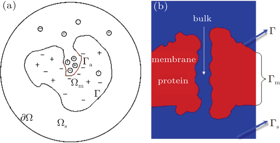 | Fig. 2. Illustrations of (a) a solvated biomolecule with active sites and (b) a channel system. |
In biomolecular systems, the concrete form of the free energy is given by

To consider the ionic size effects in ionic liquids, Andelman et al. modified the free energy form by introducing an additional solvent entropy term representing the unfavorable energy modeling the overpacking or crowding of ions and solvent molecules [ 14 ]


To account for different ionic sizes, Chu et al . extended this model to include two different sizes and gave an explicit SMPB form in the study of ion binding to DNA duplexes. [ 15 ] All the explicit forms are obtained by substituting the ion concentration of Boltzmann distribution in the PB equation with an explicit form of modified concentration after considering the ionic volume exclusion. However, an explicit form of an ion concentration as a function of the potential and ionic sizes does not exist for a general case with various ionic and solvent molecular sizes. Because the PB model (equilibrium description) can be considered as a specific case of the PNP model (non-equilibrium description), we can resort to the sizemodified PNP framework to implicitly obtain the SMPB results. We have modified the steady-state PNP equations to obtain nonuniform size-modified PNP (SMPNP) equations that naturally treat arbitrary number of ion species with different sizes and can describe both equilibrium state (i.e., PB case) and non-equilibrium processes of ionic solutions. [ 10 , 17 ] The chemical potential from the variation of the free energy in Eq. (


The classical DFT, a systematical theory to investigate inhomogeneous fluids, can be coupled with the PNP equations to improve simulation results for biomolecular systems. The major issue with DFT lies in the construction of an excess Helmholtz free energy. [ 37 ] The fundamental measure theory (FMT), derived by Rosenfeld, provides an excellent suggestion on how to construct the excess Helmholtz free energy for inhomogeneous hard sphere mixtures and has been developed and widely used in many studies. [ 21 , 38 – 46 ] According to the theory, [ 38 ] the excess Helmholtz free energy due to the hard sphere repulsion is given as follows:


In addition to the ideal chemical potential 


In contrast to the integral form of the excess chemical potential and the above mentioned efforts to solve the integrodifferential equations, Liu et al . have derived a local hard sphere description for 


In addition to the chemical potential due to hard sphere repulsions, chemical potential terms resulting from electrostatic correlations and short-range attraction interactions have also been analyzed in many studies. [ 22 , 23 , 43 ] There are also some improvements in the FMT to account for discrete particle interactions. Kierlik and Rosinberg proposed a simplified version of the FMT, which was proven to be equivalent to the original FMT but required only four scalar weight functions. [ 45 ] Using the Mansoori–Carnahan–Starling–Leland bulk equation of state, Roth et al . and Wu et al . independently published the white-bear version or the modified FMT to make simulation results more accurate. [ 40 , 42 ] For inhomogeneous fluids of nonspherical hard particles, Mecke et al . derived a fundamental measure theory using the Gauss–Bonnet theorem. [ 44 ] These different forms of the excess Helmholtz free energy lead to different expressions of the excess chemical potential and thus different coupling results of DFT and PNP.
Polar and nonpolar interactions are coupled. In recent years, a few groups used a variational framework to study the coupled system. [ 28 – 30 , 47 ] In particular, in the studies pertaining to Refs. [ 28 ]–[ 30 ], the biomolecular surface (interface between solute and solvent) was not fixed, but determined as a model output. A variational model was proposed under the consideration of an assembly of solutes with arbitrary shape and composition surrounded by a dielectric solvent in a macroscopic volume to explicitly couple hydrophobic, dispersion, and electrostatic contributions in a continuum model. The typical free energy, including volume energy, surface energy, van der Waals interaction energy, and continuum electrostatic free energy, is expressed as a functional of the characteristic function ν


In addition to the above improvements, some other modifications have also been made to the continuum model. The homogeneous assumption of dielectric medium does not coincide with the experimental results of salt water solutions. [ 48 ] We explored a variable dielectric PB (VDPB) model by considering the dielectric as an explicit function of ionic sizes and concentrations. [ 25 ] Andelman et al . proposed a dipolar PB (DPB) model by coarse graining the interaction of individual ions and dipoles. [ 49 ] A Poisson–Fermi model was derived by introducing a fourth-order free energy functional to describe the interplay between overscreening and crowding. [ 13 , 19 ] Other modifications, for example, incorporating image charge effects [ 50 ] and Lennard–Jones hard sphere repulsion [ 24 ] into the primitive model, have also been studied to improve the continuum model. Horng et al . introduced the finite size effect by treating ions and side chains as solid spheres and using Lennard–Jones hard sphere repulsion potentials to characterize this effect, and observed the ion-selectivity behavior in a simple 1D analysis and simulation. [ 47 ]
Other beyond-mean-field models have been developed at the same time to account for the ion–ion correlations. Kjellander et al . introduced the dressed ion theory, a formally exact theory for electrolyte solutions and colloid dispersions by writing the ion–ion correlation function as a sum of a shortrange part and a (relatively) long-range part. [ 51 , 52 ] For nucleic acid mixtures, the tightly bound ion theory was presented by Tan et al ., which catures the fluctuations and the electrostatic and ion–ion correlations and provides reliable predictions for ion distributions and thermodynamic properties. [ 53 , 54 ] The integral equation theory was used to evaluate the distribution functions of solvents and ions and calculate the liquid structure and thermodynamic properties. [ 55 – 59 ] In case of high valence ions, a strong coupling theory as a correction to the PB approach is available to predict the counter ion distributions around charged objects. [ 60 ] Furthermore, a system of self-consistent partial differential equations has been derived to extend the PB equation to include the electrostatic correlation and fluctuation effects, [ 12 , 61 ] and recently a numerical method was developed to solve the equations. [ 62 ]
In the simulation of biomolecular systems, progress has been made for developing more accurate and efficient algorithms. [ 1 , 31 ] In the finite difference method for the PB equation, to enforce the interface conditions and to obtain better numerical convergence, Wei et al . implemented the matched interface and boundary (MIB) method to accurately treat the interface conditions, and also used the regularization scheme described in Ref. [ 63 ] to remove the charge singularities in the molecule to achieve a higher level of accuracy. [ 64 , 65 ] Luo’s group developed the immersed interface method (IIM), a new discretization method, and implemented it in the PBSA solver incorporated in the Amber package. [ 66 ] Lu et al . used the finite element method and a body-fitted molecular surface mesh to solve the interface problem with a high level of accuracy. [ 1 , 7 ] At the same time, considerable efforts have been made to increase the speed of computations. Xie et al . employed the MPI to present a parallel adaptive finite element algorithm to solve the 3D electro-diffusion equations. [ 8 ] Geng et al . provided a GPU-accelerated direct-sum boundary integral method to solve the linear PB equation. [ 67 ] Yokota et al . presented a GPU-accelerated algorithm with the fast multipole method in conjunction with a boundary element method (BEM) formulation, resulting in strong scaling with parallel efficiency of 0.5 for 512 GPUs. [ 68 ] Lu et al . parallelized the adaptive fast multipole PB (AFMPB) package with the cilk plus system to harness the computing power of both multicore and vector processing, which achieved nearly optimal computational complexity in BEM and successfully solved on a workstation the PB equation for macromolecular systems such as a virus with tens of million degrees of freedom. [ 69 ]
We have summarized the PB/PNP types of continuum models based on the mean field approximation, their improvements to include the ionic size effects, other physical properties that have been missed in the previous models, the coupling of polar and nonpolar interactions, and numerical progress for biomolecular simulations. The main improvements for including the size effects are achieved by introducing an excess chemical potential term to account for discrete particle interactions ignored in the continuum model. However, differing from the SMPB/SMPNP models which are still based on mean field approximations, coupling of DFT and PNP provides a reliable framework for particle interactions. The variational treatment of the biomolecular surface is included in the free energy that couples polar and nonpolar interactions to obtain both an optimal surface and a minimum free energy. Numerical progress makes it possible to obtain more accurate and efficient algorithms for simulating biomolecular systems. It is expected that much effort will be made in the future for developing beyond-mean-field continuum models that can not only capture important detailed physical effects but also keep numerically tractable for biomolecular systems. At the same time, effective numerical techniques (along with advances in modern computer science and mathematics) need to be developed for dealing with larger and more complicated simulation systems.
| 1 | |
| 2 | |
| 3 | |
| 4 | |
| 5 | |
| 6 | |
| 7 | |
| 8 | |
| 9 | |
| 10 | |
| 11 | |
| 12 | |
| 13 | |
| 14 | |
| 15 | |
| 16 | |
| 17 | |
| 18 | |
| 19 | |
| 20 | |
| 21 | |
| 22 | |
| 23 | |
| 24 | |
| 25 | |
| 26 | |
| 27 | |
| 28 | |
| 29 | |
| 30 | |
| 31 | |
| 32 | |
| 33 | |
| 34 | |
| 35 | |
| 36 | |
| 37 | |
| 38 | |
| 39 | |
| 40 | |
| 41 | |
| 42 | |
| 43 | |
| 44 | |
| 45 | |
| 46 | |
| 47 | |
| 48 | |
| 49 | |
| 50 | |
| 51 | |
| 52 | |
| 53 | |
| 54 | |
| 55 | |
| 56 | |
| 57 | |
| 58 | |
| 59 | |
| 60 | |
| 61 | |
| 62 | |
| 63 | |
| 64 | |
| 65 | |
| 66 | |
| 67 | |
| 68 | |
| 69 |