2. Atomic-scale computation Atomic scale simulation is one important theoretical technique to help us understand the fundamental physics that occurs in materials science. It provides computational techniques or tools to describe the interactions among the atoms and electrons, calculate the charge distribution and charge transfer, obtain the electronic ground states and their eigenvalues, monitor the atomic movements and figure out the trajectories, and finally collect all necessary information on the materials’ physical and chemical properties at the atomic level, either from a kinetics or thermodynamics point of view. With such basic data/information, we can better understand the fundamental physical and chemical characteristics of the materials and therefore find ways to modify and design the materials from the atomic level. Generally speaking, three widely used computational methods are concerned with atomic-scale simulation: first-principles calculation, molecular dynamics (MD) simulation, and Monte Carlo (MC) simulation.
First-principles calculations deal with the ground states of the electrons in a materials system. It describes the movement of the electrons with elementary equations in many-body quantum mechanics without using any empirical parameters in the calculation. Since the development and application of density functional theory (DFT), [ 8 , 9 ] first-principles calculation provides very fast sufficiently accurate approximate solutions to the Schrödinger equation. Presently, first-principles calculation has become the core simulation technique at atomic scale. By combining it with the MD and MC techniques, most of the atomic-level physical problems that concern materials scientists can be solved. First-principles combined with MD, which was first proposed by Car and Parrinello in 1985, [ 10 ] has become one of the most important computational tools in modern materials simulation. Developing the most extensive applications in LIBs involves investigating the electronic structure of the electrode materials, the Li-ion migration energy barrier in solid materials, the energetics and the structural and electrochemical stabilities in the bulk phase and at the relevant surfaces/ interfaces, and thus analysis of electron conduction behavior, prediction of Li-ion dynamics performance and thermodynamics characteristics, and so on. However, application of first-principles calculation in designing LIB materials is not limited to the above-mentioned aspects; it includes almost all fields related to the materials’ physical and chemical properties.
MD simulation deals with the movement of classical particles (atoms, ions, molecules, etc.) in a certain macroscopic system. It solves Newton’s equation and obtains the positions and momenta of all particles in each time step, and therefore it monitors the evolution of the trajectories and energies of all particles in a certain period of time at a certain temperature. When the time span is long enough and the system approaches thermodynamic equilibrium, the statistical average over time is approximately equal to the statistical average over the ensemble. This is called the ergodic hypothesis in statistical physics, according to which the statistical average over time provides the accurate details on the structural, thermodynamic, and kinetic properties of the system. In LIBs, MD is used to simulate the Li-ion diffusion pathways and coefficient, structural evolution, and phase transition during the (de)intercalation process.
MC simulation [ 11 ] is similar to MD in terms of monitoring the movements and trajectories of the moving particles and the statistical procedures are applied to determine the physical and chemical properties of the system. However, determining how the trajectory is created or how the movement is created is done in a different way. In MD simulations, particle movement is simulated by solving Newton’s equation, while in MC, particle movement is generated in a random sampling manner. Therefore, MD is called the deterministic approach whereas MC is called the uncertainty approach. In most cases of solving physical problems using MC, the Metropolis sampling method is used. [ 12 ] The metropolis sampling is a nonnormalized sampling method, which depends strongly on the physical nature of the system. MC is a very flexible method with various applications in solving physics problems. Applications of MC simulation in the LIB field include modeling the Li-ion diffusion process, determining an electrode material’s structural stability during the charge/discharge process, calculating the phase diagram, and even predicting the intercalation potential of the electrodes at different charge/discharge stages.
Since computing power limits the size of the unit cell to roughly 10 2 atoms in first-principles calculations, [ 3 ] the applications and promotion of first-principles calculation are constrained. On the other hand, in order to obtain results that converge with respect to system size, a system consisting of millions of atoms (or more) is needed and Monte Carlo simulation has to be applied. Moreover, problems such as finding the equilibrium composition profile, building the dependence of Li-ion diffusion coefficient on the Li-ion concentration in lithium-ion battery materials, and constructing the temperature–concentration phase diagram require extensive sampling of configuration space that would be prohibitive via first-principles calculation alone. To address these issues, the cluster expansion formalism is a power tool that serves as a link between first-principles calculation and Monte Carlo simulation as shown in Fig. 2 .
The general formulism of cluster expansion parameterizes the energy as [ 13 ]
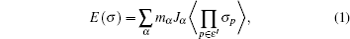
where
α denotes cluster,
p site,
ε ′ equivalent cluster of
α ,
J effective cluster interaction (ECI),
m cluster multiplicity,
σ configuration, and
σ p atoms arrangement variable. Each term in the summation of Eq. (
1 ) denotes interactions within clusters of a certain number of atoms. Take the case of binary system (concentration of component
X is variable). Cluster expansion formulated in Eq. (
1 ) could be refined as

where
J denotes ECI,
σ fundamental descriptor of crystal structure represented by the state of component
X (states of atoms
X , e.g. 1 if the site is occupied by
X and 0 if the site is unoccupied);
i ,
j , and
k are used to distinguish identical sites;
[ 3 ] J null denotes energy of an empty cluster,

of a point cluster,

of a pairs cluster, and

of a triplets cluster. Cluster scale could be enlarged. Accordingly, terms in Eq. (
2 ) would be increased. That would be more beneficial in obtaining the energy, approaching the result of first-principles calculation. The computation result is also affected by the accuracy of ECI, which could be known through experiments or first-principles calculation.
An early application of the cluster expansion method was in the theoretical prediction of ordered superstructures in metallic alloys by Sanchez and de Fontaine in 1981. By assuming a certain set of ECIs, they examined the consequences in the configurational energy of binary alloys and found all the superstructures that could be ground states for a certain type of ECI. [ 14 ] Also, de Fontaine et al. applied the cluster expansion method in the construction of the Ti–Rh phase diagram and the O-ordered phase diagram of YBaCuO at the end of the 1980s. [ 15 – 17 ] From then on, the cluster expansion method has often been combined with first-principles calculation and Monte Carlo simulation to be applied in the investigation of a material’s thermodynamics and kinetic behaviors, in which supercells including millions of atoms are usually used to approach the reality.
In the rest of this section, we review how atomic-scale computations are used in modifying and designing new LIB materials, predicting new features of the materials and giving theoretical guidance to the experiments.
2.1. Electronic structure The electronic structure is the most important characteristic of a solid material: most of the physical and chemical properties of a solid material are strongly associated with the electronic structure. Based on DFT, first-principles calculation provides a convenient tool to calculate and analyze the electronic structures of crystalline materials. When the electronic structure is obtained, many other properties can be derived by simple physical or mathematical analysis. Currently, a variety of computational codes have been developed to calculate the electronic structures, including the Vienna ab initio simulation package (VASP), [ 18 ] the Cambridge sequential total energy package (CASTEP), [ 19 ] DACAPO, [ 20 ] the quantum Espresso, [ 21 ] etc. Generally, these codes use the Vanderbelt ultrasoft pseudopotentials [ 22 , 23 ] or projector augmentedwave method, [ 24 ] and the wave functions are expanded with plane wave basis sets. Within the DFT scheme (and sometimes also post-DFT such as hybrid functional, GW method random phase approximation, and so on), these codes solve the Kohn–Sham equation and obtain the eigenstates and energy eigenvalues. With these eigenstates and energy eigenvalues, both the energy band dispersion in the k -space and the charge distribution in real space can be analyzed. For convenience, we always plot the energy band structure which gives the energy band dispersion curve along a specific line (direction) within the first Brillouin zone in the k -space.
First-principles calculation of the electronic structure can be used to predict the electronic conduction behavior of the electrodes. For example, LiFePO 4 is an important cathode material first proposed by Goodenough et al . [ 25 ] The low intrinsic electronic conductivity of the LiFePO 4 compound results in very poor rate performance when it is employed as a cathode for an LIB. Using first-principles calculation, Shi et al. predicted that a small amount of Cr doping at Li sites would change the electronic structure of LiFePO 4 from insulating to half-metal, and thus suggested that Cr doping can enhance electronic conductivity substantially. [ 26 ] The LiFePO 4 cathode is not the only case: first-principles also identified that the electronic conductivity of LiCoO 2 can be enhanced through Mg doping at its octahedral sites. [ 27 ] On the other hand, first-principles calculation can also predict the electronic conduction changes upon lithiation [ 28 ] or delithiation [ 29 ] of an electrode.
Although the DFT within the local density approximation (LDA) or generalized gradient approximation (GGA) already shows feasibility in predicting the electronic conduction behavior of LIB materials; calculation always substantially underestimate the band gap, particularly for the cathode materials that contain strongly localized electrons at the 3d states of the transition metal oxides. Hence, we need post-DFT calculations to give better predictions of the electronic structure of the cathode materials. Hybrid functional is one typical improvement to the DFT. The hybrid functional uses a fraction of the Hartree–Fock (HF) exchange energy plus a fraction of a conventional semilocal functional, and has been shown to be able to represent the electron localization effect in the transition metal oxide cathode materials. Using the Heyd–Scuseria–Ernzerhof (HSE06) [ 30 – 33 ] hybrid functional, Chevrier et al. [ 34 ] showed that the HSE06 hybrid functional can give a very good prediction of the electronic structures and energetics of transition metal oxide cathodes. However, the computational efficiency is very low compared with that of the LDA/GGA level calculations. Alternatively, DFT+U is a better choice in determining the band gap of insulating materials. Within the DFT+U calculation, the high efficiency of the LDA/GGA is inherited while the localization effect of the 3d states is treated by including a Hubbard U term to describe the Coulombic onsite effect. [ 35 , 36 ] Using the DFT+U, the band gap of LiFePO 4 is predicted to be 3.7 eV, [ 37 ] in good agreement with experimental value (3.8 eV) while much better than the GGA predicted 0.53 eV. [ 26 ]
The correct description of electron localization is very important in the simulation of transition metal oxide cathode materials. For example, a strong Jahn–Teller (JT) effect occurs in the LiMn 2 O 4 cathode. When the Mn is in the oxidation state of Mn 3+ , the MO 6 octahedral is severely distorted with two Mn–O bonds elongated and the other four shortened, due to the JT effect. However, the JT effect cannot be represented in first-principles calculations without the correct description of the electron localization effect of the Mn-3d states. Therefore, DFT results at the GGA or LDA level do not reproduce the JT distortion in the LiMn 2 O 4 compound, and the electronic structure is predicted to be metallic as shown in Fig. 3(a) , which is obviously not correct. In contrast, DFT+U calculation can give good description of the localized electrons at the transition metal atoms’ 3d states, and therefore the electronic structure (see Fig. 3(b) ) and the Jahn–Teller distortion can be well represented. [ 38 ] Once the electronic localization effect is well described, we can study the character of the small polaron states in the cathodes. A polaron state is a localized state with charge carriers constrained in a certain local atomic environment. The polaron state is always associated with local atomic structure distortion due to the polarization effect of the localized charge upon certain atoms. Therefore, technically we can simulate the polaron migration through transferring the localized charge from one transition metal ion to another and simultaneously the distortion of the local structure also passes from one transition metal ion to another. In this way, the small polaron migration energy barrier can be calculated using firstprinciples calculation. For example, Maxisch et al. [ 39 ] studied the polaron migration in Li x FePO 4 and proposed another electronic conduction mechanism in the olivine compound. In this view, the transferring of the local atomic displacement and lattice distortion associated with the localized electron can be simulated with the nudged elastic band (NEB) method. [ 40 ] For example, Ouyang et al. calculated the JT-type small polaron migration in the LiMn 2 O 4 compound, [ 41 ] and they also predicted that the polaron migration energy barrier is very sensitive to external strain applied to the lattice. [ 42 ]
2.2. Lithium-ion dynamics Lithiumion dynamics is a very important factor for evaluating LIB materials. Good Li-ion diffusivity in both electrode and electrolyte materials is desired in order to achieve good rate performance. Generally, the diffusion coefficient is the most important parameter to characterize the Li-ion diffusion dynamics. The macroscopic Li diffusion behavior is governed by Fick’s law of diffusion,

where
C ,
D c , and
t are the concentration of diffusion particles, the chemical diffusion coefficient, and time, respectively. Obviously, it is difficult to calculate the chemical diffusion coefficient directly from Fick’s law via atomic scale simulation, because the variation of concentration over time is difficult to determine by either MD or MC simulation, both of which are based on a theorem from equilibrium statistical physics. Furthermore, Fick’s law does not help one understand the diffusion mechanism, which is always associated with microscopic Li migration behavior. On the other hand, a tracer diffusion coefficient can be used to describe the diffusion behavior at atomic scale. Experimentally, we can trace the atomic motion trajectory via monitoring the movement of isotopic atoms, and then the tracer diffusion coefficient can be calculated via

where
N denotes the number of moving particles,
t is the time, and
r i (
t ) is the position of the
i -th particle at
t . In order to measure the tracer diffusion coefficient, the time span of the measurement should be long enough in order to have a good statistical sample of the particles’ movements, which increases experimental expenses. However, computer simulation can do this job well at low expense and with much higher efficiency. MD and MC can simulate the particles’ movements under certain external conditions and record the motion trajectory, giving an observation of the diffusion behavior that is similar to an observation based on tracer isotopic atoms. MD/MC simulations can be performed at different temperatures and the diffusion coefficient varies with the temperature and the relationship between the diffusion coefficient and the temperature obeys Einstein’s relation, with which we can evaluate the diffusion activation energy.
The diffusion activation energy is equal to the statistical average of a particle’s migration energy barrier in solid-state materials. On the other hand, we can also calculate it directly from atomic scale simulations. First-principles calculation combined with the nudged elastic band (NEB) method provides a convenient approach to optimize the migration pathway directly and to calculate the energy barrier. Shi et al. reported that Li + vacancies in Li 2 CO 3 diffuse via a typical direct hopping mechanism. However, as for the excess Li + interstitials’ diffusion, they suggested that the transport energy barrier is significantly lower if a moving Li + sees a series of transition states with five- or four-coordinated O-ligands. This would happen only when this Li + replaces another Li + in its original position, as shown in Fig. 4(a) , which is called the knock-off mechanism; in any other case, a longitudinal direct diffusion would encounter much higher energetic barriers (see Fig. 4(b) ). [ 43 , 44 ]
With the energy barrier from first-principles NEB calculation, we can evaluate the self-diffusion coefficient using the lattice gas model [ 45 , 46 ] within the hopping mechanism. The self-diffusion coefficient can be expressed as

where
a is the hopping distance of the migrating particle in the lattice,
ν is the vibration frequency of the hopping particle,
E a is the migration energy barrier from the first-principles NEB calculation,
k B and
T are the Boltzmann constant and the absolute temperature, respectively.
Atomic scale simulation of Li-ion diffusion behavior uses the MD/MC method to calculate the mean square displacement and the first-principles method to calculate the Li-ion migration energy barriers in the solid electrode and electrolyte materials. In both cases, the self-diffusion coefficient can be evaluated conveniently. From these atomic scale simulations, the Li-ion diffusion mechanism can also be identified, which helps to modify and design materials’ properties. Here we take LiFePO 4 cathodes as an example, from first-principles calculation and MD simulation, it is identified that Li diffusion in the LiFePO 4 cathode is along a one-dimensional diffusion channel with an energy barrier of about 0.6 eV. [ 47 ] This gives a reasonable explanation of the limitation of the Li site doping strategy, which is expected to improve the intrinsic electronic conduction of the olivine compound. By using first-principles molecular dynamics simulation, Shi et al. studied the ion transport mechanism in solid electrolyte LiI(C 3 H 5 NO) 2 , and found that LiI(C 3 H 5 NO) 2 is a unique iodine-ion conductor. This conclusion challenges the common intuition that the diffusion conditions favor Li + ions due to lithium’s lighter mass, but it does agree with the available experimental data. [ 48 ] Furthermore, MC simulation can numerically evaluate the effect of Li site doping in blocking the one-dimensional diffusion pathway. [ 49 ]
MC simulation is also widely used to study the Li-ion dynamics in electrode materials. When MC simulation is applied to study Li-ion dynamics, the most important and difficult task is to figure out the interactions between moving Li ions and the lattice in which the Li ions are accommodated. However, if a reasonable interaction model is constructed, MC simulation can give a very good prediction of the Li-ion diffusion behavior. For example, Newman et al. [ 50 ] studied the Li diffusivity in a LiMn 2 O 4 cathode and reproduced the experimental observations with a simple interaction model, which was established by Dahn et al. [ 51 ] in order to study the voltage of this spinel compound. With a similar interaction model, Ouyang et al. studied the Li-ion conductivity in LiMn 2 O 4 at various temperatures. [ 52 , 53 ]
An interaction model or interaction potential function is also very important in classical MD simulations. There is little literature available reporting on classical MD simulation of Li-ion dynamics in LIB materials particularly cathode materials. The reason lies in the fact that the interactions among Li ions, transition metal ions and O are very complicated and it is very difficult to figure out a reasonable model to describe these interactions. Suzuki et al. and Tateishi et al. [ 54 , 55 ] developed an empirical potential function for LiMn 2 O 4 , but their MD results are not consistent with the experimental data. Therefore, most MD simulations on LIB materials employ Car Parrinello MD (CPMD), [ 10 ] which is based on density functional theory. Using the CPMD, Ouyang et al. [ 56 ] gave a reasonable prediction of the Li migration energy barrier of about 0.23 eV in a LiMn 2 O 4 cathode.
2.3. Lithium intercalation potential and energetics Energetics is particularly important for LIBs because the major function of a battery system is to store energy. The output energy of a battery system originates from the Gibbs free energy change upon Li moving from the anode side to the cathode side. The Gibbs free energy value can be obtained from atomic-scale simulation and therefore, we can calculate the output voltage of a battery system. As the electrode materials for LIBs are all in solid state, we can assumed that the entropy and volume changes during Li insertion/extraction reactions are small and their contribution to the Gibbs free energy is negligible, so the average intercalation potential can be calculated directly using the ground state total energy value from first-principles calculations. [ 57 ]
The intercalation potential is a key feature of any electrode material for lithium-ion batteries. First-principles calculation predicts the intercalation potential and therefore helps us discover new materials for LIBs. We can calculate the intercalation potential for a large number of Li compounds and select potential cathode and anode materials according to the calculated intercalation potential. For example, Ceder et al. studied hundreds of materials that contain X O 4 ( X = P, S, As, Si) [ 58 ] by high-throughput first-principles calculations and discovered some novel cathode materials with high capacity and high intercalation potential. Shi et al. developed a method based on density functional theory to study the physics of defects in a solid electrolyte in equilibrium with an external environment. This method was successfully applied to predict the ionic conduction in Li 2 CO 3 [ 43 , 44 ] and LiF, [ 59 ] in contact with different electrodes which serve as reservoirs with adjustable Li chemical potential ( μ Li ) for defect formation. The structural stability of an electrode material, particularly during the processes of Li insertion and extraction, is important to its cycling performance. For example, the theoretical capacity of a LiCoO 2 cathode is ∼ 274 mAh/g after removal of all Li ions from the compound. However, the practical capacity is only about 140 mAh/g, that is, only a little more than half of Li ions can be extracted from the cathode side. When more than half of the Li ions are removed from the LiCoO 2 compound, its layered structure becomes unstable, phase transition occurs and the newly formed phase is no longer electrochemically active. The energetics of the phase transition can also be predicted from atomic-scale simulations. In these studies, approaches that combine first-principles calculation with kinetic MC simulation are always used. First-principles calculation gives the ground state energy of a compound at different intercalation stages, and then these energies are used as input for MC simulations, in which the cluster expansion technique is applied. With this strategy, van der Ven et al. studied the phase ordering of LiCoO 2 cathodes and calculated the phase diagram at different charged stages. [ 60 ] In 2001, by parameterizing the activation barriers obtained from first-principles calculation with a local cluster expansion and applying the result in kinetic Monte Carlo simulations, van der Ven et al. proposed that lithium diffusion in layered Li x CoO 2 is mediated by divacancies at any concentration of lithium. Furthermore, because the height of the activation barrier depends heavily upon the concentration of lithium, the predicted diffusion coefficient varies by several orders of magnitude with lithium concentration x . [ 61 ] By combining Hubbard-U-corrected (GGA+U) density functional theory in the generalized gradient approximation with cluster expansion and the Monte Carlo simulation technique, Hinuma et al. obtained the temperature–concentration phase diagram for Na x CoO 2 (0.5 ≤ x ≤ 1), which agrees well with experimental results. [ 62 ] Using first-principles calculations, Malik et al. studied the effect of cation substitution on the transition-metal sublattice in phospho-olivines, with special attention given to the Li x (Fe 1 − y Mn y )PO 4 system. Then a cluster expansion model was derived from first-principles with Monte Carlo simulations to calculate finite- T phase diagrams, voltage curves, and solubility limits of the system. [ 63 ] Ong presented an efficient method of characterizing from first principles the phase diagram of the Li–Fe–P–O 2 system as a function of oxidation conditions. By incorporating experimental thermodynamics data, they also constructed a modified Ellingham diagram to visually represent the relation between temperature, oxygen partial pressure, and the chemical environment necessary to achieve a desired reduction reaction. Ong proposed that the methodological approach developed can conceivably be extended to any system of interest. [ 64 ]
To investigate structural stability, calculation of the lattice dynamics is another aspect. Based on the first-principles total energy calculation, we can calculate the inter-atomic forces with the Hellmann–Feynman theorem and then the dynamic matrix can be derived. With these data we can obtain the phonon frequency and the phonon dispersion curve of solid materials. If the structure is in a local minimum, which corresponds to a stable (meta-stable) state, the phonon frequency is a real number. On the other hand, if the structure is not in a local minimum, imaginary phonon frequency will appear at certain q -states. Therefore, the structural stability can be judged by calculating the phonon dispersion spectrum.
Two atomic-scale simulation methods are used to calculate lattice dynamics: the force constant method and linear response theory. The literature shows that both methods are widely used. For example, the phonon data of LiFePO 4 compound are calculated from the first-principles force constant method. [ 65 ] After the phonon data are calculated, the lattice vibration entropy’s contribution to the free energy can be evaluated. In general, the entropy contribution is so small as to be negligible. However, recent results show that vibrational entropy’s contribution to the free energy of a LiCoO 2 cathode is around 0.2 to 0.3 eV, so vibrational entropy’s contribution to the intercalation potential of the LiCoO 2 cathode can be as high as 95 mV at 300 K, as shown in Fig. 7 . [ 66 ]
2.4. Combination of first-principles calculation & transmission electron microscopy Transmission electron microscopy (TEM) is among the most robust means of nanocharacterization, with higher resolution ( δ ) than the visible light microscope (VLM), but both are limited by wavelength, according to the Rayleigh criterion:

The wavelength
λ of the radiation in TEM (
λ = 1.22/
E 1/2 ,
E is in electron volts, and
λ in nm, by Louis de Broglie) is much shorter than that in VLM, resulting in its higher resolution. Here,
μ is the refractive index of the viewing medium, and
β is the semi-angle of collection of the magnifying lens.
Besides decreasing λ by increasing E , which aims to push the resolution limit, other tactics to improve the resolution include spherical aberration and chromatic aberration, both allowing sharper atomic resolution of images. The former permits the generation of a finer electronic beam with denser currents, yielding better spatial resolution; however it requires a sufficiently thin specimen for proper depth of field. In contrast, the latter is used to improve the image quality for thicker specimens. The combination of intermediate-voltage electron microscopes and spherical aberration correction can lead to atomic resolution below the 1 Å threshold, which directly contributes to building convincing models for atomic-level calculations, such as those based on first principles. The images of scanning transmission electron microscopes (STEM) are magnified by the scan dimensions on the specimen rather than by the lenses (lenses magnify in TEM), promising higher magnification and sub-angstrom resolution without the stringent specimen thickness requirement. In addition, annular-brightfield (ABF) favors the lighter elements such as lithium. All the improvements above contribute to the direct observation of Li, which is of critical importance for investigating Li-ion batteries. [ 67 ]
Direct images of samples can help to reveal the microscopic mechanisms of Li ions’ distribution and storage, [ 68 , 69 ] (de)lithiation induced phase transformation, [ 70 – 74 ] stress and strain, [ 75 ] surface, [ 76 , 77 ] and interphase, [ 78 ] evolution, nearly equilibrated state after electrochemical cycling, [ 79 ] kinetic performance, [ 80 ] and so on, which are among the major issues in calculations. However, some limitations of TEM remain: (i) the ionizing radiation damages the specimen, particularly low-electronic conductive samples such as solid electrolytes; (ii) the higher resolution corresponds to worse sampling ability (the vein of a leaf but not the whole forest is focused on); (iii) images from TEM are the two-dimensional projection of actual three-dimensional samples without enough depth sensitivity, and hence are probably misleading. Consequently, the calculations can be a necessary complement to TEM, for the following reasons: (i) calculations’ universality for both conductive and nonconductive materials; (ii) the convenience to build up and analyze periodic models and relate the microscopic structure to the macroscopic performance; (iii) the ability for building up nonperiodic models, such as surface and interphase models, to examine and explain the 2D images.
By combining first-principles calculation and direct atomic-scale observation by ABF-STEM, Yue et al. [ 81 ] reported two distinct guest ion occupation paths in the orthorhombic Fe 2 (MoO 4 ) 3 electrode – a discrete one for Li and a pseudo-continuous one for Na – as well as their relationship with single-phase and two-phase modes for Na + and Li + , respectively, during the intercalation/deintercalation process.
3. Phase-field modeling Compared with first-principles calculation, MC and MD simulations at the atomic-scale, phase-field (PF) modeling has a wider span, from atom scale to continuum scale, so it has become a basic paradigm to simulate materials’ kinetic behaviors. However, it is still reasonable to think of PF as a mesoscale method, since its modeling is semi-phenomenological and its theoretical basis is established from thermodynamics, elasto-plastic mechanics, electrochemistry, etc. So far, even if the existent PF models in themselves cannot account for all the interesting physical and chemical factors within a microstructure, a large number of applications of PF in materials communities, such as ordering, [ 82 ] dendritic growth, [ 83 ] crack propagationm, [ 84 ] martensitic transformation, [ 85 ] and precipitation. [ 86 ] have been realized, which covers almost all kinetic simulations of materials at mesoscale. Following the emergence of novel physical or chemical models, PF is very promising for more applications. At present, the development of PF depends on three factors: physical or chemical modeling, industrial requirements and database. First, the physical or chemical modeling is the basis of PF modeling, giving a consistent PF frame of materials’ kinetics problems, such as diffusion, stress distribution, chemical reaction, and so forth. Once a PF model is built that describes materials’ kinetics behaviors, the results of PF simulation enable one to explain several perplexing problems in the processes of transformation, diffusion, etc., and to validate the reliability of the physical or chemical models. On the other hand, the aim of PF modeling is generally to help engineers design material engineering procedures and analyze microstructural changes that might occur during processing, all of which is closely associated with the industrial requirements. Certainly, some applications of PF modeling, such as solidification [ 87 ] and precipitation, [ 88 ] have entered industrial practices to interpret the topography of dendritic or grain growth, multicomponent diffusion, precipitation behaviors, etc., benefiting from the linkage between the CALPHAD (calculation of phase diagram) method and PF modeling. CALPHAD offers the set of the thermodynamic parameters needed by PF modeling. For different alloy systems and transformation patterns, a database plays an important role, providing the basic data sets to adapt the PF model to industrial conditions. For example, CALPHAD has been linked to PF modeling successfully to satisfy industrial requirements of simulating alloy precipitation [ 88 ] and solidification [ 87 ] for multicomponent alloy systems.
The underlying physical concepts of PF modeling can be traced back to the classic work of Gibbs [ 89 ] and Cahn et al. , [ 90 ] who respectively constructed the basis of the thermodynamics and the diffusion-interface description. Phase-field modeling is based on the diffusion-interface description, so the PF parameters vary continuously and smoothly in the two-phase interface range with no sudden change. Temporal microstructure evolution is described by a pair of well-known continuum equations, namely, the Cahn–Hilliard nonlinear diffusion equation [ 91 ] (7) and the Allen–Cahn (or time-dependent Ginzburg–Landau) equation [ 92 ] (8) toward conservative and non-conservative field variables,


where
c and
η stand for the conservative and non-conservative field variables, respectively, which characterize transformation behaviors;
M i is the diffusional mobility of the
i th component; and
L i j is the kinetic matrix related to interface mobility. For instance, bulk composition belongs to the conservative field variable, whereas the order parameter characterizing constituent phases belongs to the non-conservative field variable. These two kinds of variables describe the features of the constituent phases. Total free energy functional
F can be expressed as the sum of various energetic terms, such as chemical energy
E chemical , interface energy
E interface , elastic energy
E elastic , and so on,

In this way, the complex interaction between phases can be handled by adding new terms to Eq. (
9 ), which is another advantage of PF modeling. That is, other physical or chemical factors can be introduced into PF model by only adding corresponding terms to Eq. (
9 ).
Generally speaking, the PF method enables one to construct a pattern for calculating the phase-transformation kinetics. Currently, the basic forms for phase-field modeling and subsequent calculations have been set; the standard steps can be summarized as follows: first, define the conservative or non-conservative parameters to characterize physical models for concrete problems; and then construct the total free energy functional to match the chemical, interfacial, and elastic features of system; finally, obtain microstructural evolution by solving the governing equations.
The earliest PF modeling was used mostly to solve the problems possessing isotropic properties, regardless of the effects of complex physical or chemical factors. Following the emergence of novel theories [ 93 , 94 ] and various physical or chemical models, PF modeling has enabled more complex problems, like anisotropic interfaces, elasto-plasticity, and chemical reactions, to be solved.
Following developments in physical and chemical models, the PF method has also been applied to aspects of LIBs such as Li metal electrode electrodeposit [ 95 ] and phase separation [ 96 ] and stress distribution [ 97 ] during Li-ion intercalation/ deintercalation. Compared with ordinary PF modeling, some difficulties have to be overcome when it is used in the LIBs, because the influences of electrode/electrolyte reaction, overpotential, phase separation, coherency strain, etc. pose various problems such as non-equilibrium, nonlinearity, charge transfer, and coupling among different factors. But some notable improvements have been made for the application of PF modeling in studying LIBs. The applications involving phase separation and coherency strain are often confined at mesoscopic lengths and at time scales beyond the reach of molecular dynamic and bulk continuum models. At present, some PF simulation results agree well with experimental data. Details of successful applications are discussed in the next three subsections, including electrochemical processes, interactions between diffusion and mechanics, and other applications.
3.1. Electrochemical processes Charge and discharge of LIBs correspond to the electrochemical process of Li ions migrating repeatedly between anode and cathode materials. One of the key problems influencing LIBs performance lies in the choice of electrode materials, which involves the materials’ response to applied voltage and current. There are special rules for anode and cathode materials: anode materials are required to possess better chemical compatibility with electrolytes, thermodynamic reversibility, chemical stability during lithiation, as well as mild reaction kinetics; cathode materials need to exhibit the lower free energy change during Li deintercalation, fast diffusion, reversibility during the deintercalation reaction and high conductivity.
During the electrode reaction, Li-ion transport plays an important role and brings about a number of problems, such as phase separation, [ 98 ] elastic coherency strain, [ 99 ] reaction limitation, [ 100 ] crystalline anisotropic transport, [ 101 ] and interfacial energy. [ 102 ] Some complex factors in LIBs are beyond the scope of classical electrochemical kinetics. For example, the Butler–Volmer (BV) equation is confined to the dilute solution approximation; the Marcus theory of charge transfer likewise considers isolated reactants and neglects elastic stress, configurational entropy, and other nonidealities in condensed phases.
The shortcomings of the classical theories leave us with difficulty in explaining some microstructural phenomena. A representative example is the Li-ion battery material Li x FePO 4 (LFP), [ 96 ] which strongly tends to separate into Li-rich and Li-poor solid phases. Experiments reveal stripe phase boundaries on the active crystal facet, rather than the isotropic “shrinking-core” within each particle that a chemist found when he simulated the phase separation in LFP; [ 98 ] the reaction rate at a surface undergoing phase transformation was his focus. These results imply the importance of phase separation and surface modification in LFP. However, classical battery models cannot represent the roles of phase separation and surface modification.
Following the effects of electrochemical thermodynamics on the concentration of solutions and on nonequilibrium systems, and integrating these effects into the PF model, PF modeling could offer more kinetic information to help one understand the electrochemical behaviors and even find ways of improving electrode performance. The first electrochemical PF model was proposed by Guyer et al. [ 103 , 104 ] Under a set of assumptions, such as ideal solution thermodynamics in bulk, the model captures the charge separation at the electrochemical interface and analyzes the conditions for electrodeposition and electrodissolution processes. Gathright et al. extended Guyer’s model to study the electrochemical impedance spectroscopy behavior. [ 105 ] Deng et al. [ 106 ] extended Guyer’s model to represent the formation of a solid electrolyte interface (SEI) layer on the anode surface. They treated it as a phase transformation process driven by the electrochemical reaction at the SEI/electrolyte interface. In these models, an electrostatic energy term was introduced into the free energy functional, and a Poisson equation ( 10 ) was applied to calculate the electric potential,

where
ɛ (
ξ ) is electrical permittivity,
ϕ is electrostatic potential, and
ρ is charge density. By putting the free energy functional into the Cahn–Hilliard equation (
7 ) and Allen–Cahn equation (
8 ), the distributions of composition and phase field over time will be obtained. Such a PF model is applicable to deal with the solid–liquid interface, but it ignores the phenomena involving the solid phase transformation.
With the development of electrochemistry, especially on the chemical kinetics of a solution’s concentration and the charge transfer theory based on non-equilibrium thermodynamics, phase field modeling has been successfully applied to various electrochemical processes such as microstructural simulations of phase separation [ 96 ] and surface nucleation. [ 107 ] This initial idea was born by combining the charge relaxation model in concentrated electrolytes [ 108 , 109 ] and Cahn–Hillard (CH) model for Li x FePO 4 . [ 110 ] The formula derivation of electrochemistry and PF can be found in the paper of Bazant et al. , [ 94 ] who modeled the non-equilibrium thermodynamics of electrochemistry and improved the electrochemical theory for the phenomenon of solution concentration. Furthermore, they introduced the charge-transfer theory [ 111 ] with statistics, [ 112 ] and nonequilibrium thermodynamics [ 113 – 115 ] into a phase field model. [ 94 ] Surrounding the LiFePO 4 , Bazant et al. carried out a great deal of research by modified phase field models. [ 94 , 96 , 100 , 107 , 109 , 116 , 117 ]
Nanoparticles of LiFePO 4 have been instrumental in building batteries that demonstrated ultrafast discharge [ 118 ] and high power-density carbon pseudocapacitors. [ 117 , 119 ] Nevertheless, given the highly anisotropic transport, [ 101 ] sizedependent diffusivity [ 101 ] and the strong tendency to separate into Li-rich and Li-poor phases, [ 120 ] the rational design of such battery systems needs to take into account the LFP’s electrochemical process and reaction kinetics, which include standard thermodynamics, phase transformation, and Li intercalation/ deintercalation kinetics, and especially, the response to applied voltage and current. Several PF modeling results enable in-depth understanding of experiments. In 2007, Bazant et al. were first to report PF kinetics with Cahn–Hilliard reaction (CHR) and Allen–Cahn reaction (ACR) models with consideration of the electrochemical reaction; [ 100 , 121 ] they modified Poisson–Nernst–Planck(PNP) equations, [ 122 ] then modified the generalized BV equation [ 109 ] in 2009, and finally formulated a complete theory [ 117 , 123 ] in 2011. As for the electrochemical applications of phase field modeling, Burch et al. studied the intercalation of Li ions in nanoparticles, [ 116 ] conducting early simulations of “mosaic instability” in collections of bistable particles. [ 124 ] Tang et al. [ 125 , 126 ] used the phase field model to simulate the phase separation and crystalline-to-amorphous transformation in spherical isotropic LiFePO 4 particles, which prompted experiments to seek the predicted amorphous surface layer. [ 127 ] The galvanostatic discharge simulation by Bai et al. presented an unexpected prediction of a critical current for the suppression of phase separation [ 117 ] as well as spinodal decomposition with a voltage plateau. Stanton et al. modeled anisotropic coherency strain [ 128 ] and obtained a stripe morphology in the equilibrium state of Li x FePO 4 . Using parameters from first-principles calculation, Cogswell et al. predicted the phase behaviors in LFP and the critical voltage for nucleation [ 107 ] through PF modeling, with results that are in excellent agreement with experiments. Moreover, Ferguson et al. [ 129 ] were first to model the phase separation in a porous electrode.
In order to help the reader understand PF modeling functions, an example is discussed here in detail. Cogswell et al. employed the Allen–Cahn reaction model to study the kinetics of phase separation in LFP nanoparticles. [ 96 ] They introduced the regular solution model considering the coherency energy and validated it by the calculated and measured LFP solubility as a function of temperature and particle size. Their results indicate that the {100} stripe morphology appearing during the phase separation is realistically simulated by phase field, in agreement with the HRTEM [ 130 ] and TEM results, [ 98 ] whereas the {101} stripe morphology was exhibited when coherency was lost in the {001} direction  (Fig. 11 ). The interface width obtained by PF modeling is close to 12 nm, which is comparable with the STEM/EELS results. [ 120 ] Furthermore, the galvanostatic discharge simulation shows that the coherency strain significantly suppresses phase separation during the discharge and leads to upward-sloping voltage curves for single particles below the critical current. According to the stripe wavelength, PF modeling gives a small interface energy γ =39 mJ/m 2 between Li-rich and Li-poor phases, which suggests that nucleation may play a limited role in the phase transformation process. Instead, coherency is believed to be the reason that LiFePO 4 nanoparticles have greater rate capability and cycle life. Anyway, it can be seen from this example that PF can simulate the influence of complex factors, clarify some perplexing phenomena and even provide some important parameters to explain experiments.
3.2. Interaction between diffusion and mechanics Failures determine the length of LIBs’ lives. In general, the reason for LIB failure can often be attributed to the interaction between diffusion and mechanics in the electrode material. On one hand, the intercalation of lithium into the host material can lead to drastic volumetric strain [ 131 ] and enhance stress distribution. On the other hand, due to thermodynamics, the mechanical stress contributes to the driving force for diffusion, so in turn, diffusion brings about a partial relaxation of stress, reversing the direction of the interaction between diffusion and mechanics. [ 132 ] Therefore, some quantitative physical models have been proposed [ 133 – 135 ] to explain that relationship. The exploration of the interaction between diffusion and mechanics by PF modeling can be traced back to Gurtin’s [ 136 ] work, which established a thermodynamic framework coupled with mechanics, based on the so-called microforce balance. Han et al. [ 110 ] introduced a phase-field model to describe the lithium-ion diffusion process in a storage material for LIBs, although no coupling with mechanics is represented in this model. Tang et al. [ 125 ] used a PF model coupled with mechanics to study the amorphization of nanoscale olivines. Those early attempts were focused on coupling the PF method with a linear elasticity model proposed by van de Ven et al. who investigated the effect of coherency strains on phase stability in LiFePO 4 . [ 137 ] Huttin et al. performed a simulation of stress evolution in Li x Mn 2 O 4 cathode particles using a coupled PF method for representing diffusion and mechanics. [ 138 ] Bazant et al. developed a thermodynamically consistent PF model, coupled with a representation of linear elasticity, to simulate the nonlinear Butler–Volmer reaction kinetics. [ 94 , 96 ]
Besides the linear elastic model, some elasto-plastic models have been reported. Anand et al. proposed a general formalism coupling PF method with large elasto-plastic deformation. [ 139 ] Subsequently Di Leo et al. implemented this formalism with a numerical approach to simulate the elastoplastic deformation of LiFePO 4 electrode material. [ 140 ] Chen et al. [ 97 ] studied the evolution of phase, morphology and stress in crystalline silicon (Si) electrodes during lithium insertion, obtaining the concentration and stress profiles as well as deformation geometries. Their results indicate that as lithiation proceeds in a Si electrode, the hoop stress can change from an initial compression to tension in the surface layer, which explains the experimentally observed surface cracking. Also, as shown in Fig. 12 , the stress profiles of the phase interfaces determined by phase-field modeling can be compared well with stress profiles determined by using the nonlinear diffusion model. [ 97 ]
3.3. Other applications Besides the above two applications, the PF method can be extended to some other aspects of LIBs, which demonstrates its versatility. In this subsection, we present two specific examples, i.e., crack propagation and dendrite growth.
One example is the problem of crack propagation and facture in materials. In this aspect, PF modeling for the fracture process offers a self-consistent description of brittle fracture in both the quasi-static and dynamic regimes of crack propagation. This is because PF modeling can capture the main features of crack propagation, including the Griffith criterion for crack initiation and the principle of local symmetry predicting the pathway of the cracks. In Refs. [ 141 ]–[ 144 ], the PF method was used to construct a multi-field problem model which couples the displacement with electrical potential and the fracture phase field. Very recently, Zuo et al. performed PF simulation for a Si thin-film electrode by coupling lithium diffusion and stress evolution with crack propagation. [ 145 ] Their results show that, owing to higher hydrostatic stress, lithium accumulates at the crack’s tip, and a reaction among multiple cracks takes place.
The other example is lithium dendrite formation in LIBs. Although the PF investigation of dendrite growth has been ongoing for decades, charge transport was not included in the model. Under the high overpotential and high charging rate, the electrochemical kinetics is highly nonlinear, the rate of change of a phase field is not linearly proportional to the thermodynamic driving force. In order to predict the lithium dendrite growth at an electrode-electrolyte interface, Zhang et al. developed a nonlinear PF model, in which the Butler–Volmer type electrochemical kinetics was automatically reproduced at the moving diffusion interface and a modified Poisson–Nernst–Planck (PNP) equation was used to solve for ionic transport and local overpotential variation. [ 95 ] Figure 13 shows the distributions of order parameter, Li + concentration and electric potential for lithium dendrite. The deep red and blue regions represent the higher and lower values, respectively. The distribution of order parameter reveals the morphology of lithium dendrites in the electrodeposit process. The distribution of Li ions indicates that higher concentration occurs in the liquid phase and there is a transition between the composition of the liquid and that of the dendrite trunk. The distribution of electric potential reflects that the transition of electric potential approximates a flat plane, being just as sensitive at the dendritic tip. This information is useful in controlling Li + electrodeposition technology.
Here at the end of this part, it is worth emphasizing that PF mainly relies on progress in the development of physical, chemical and mechanical models, which implies the importance of a thermodynamics database and a suitable elastoplastic scheme. Also, it is important to keep in mind that PF modeling, first-principles calculation and the continuum bulk method are not isolated, but are interwoven with each other. A set of parameters in the PF model, including formation enthalpy, interface energy, chemical reaction barrier, elastic constants, etc., can be obtained from first-principles calculation. In addition, if a phase-field model is based on lengths close to or larger than micrometer scale, or it involves treating a free-boundary condition, the finite element algorithm that is suitable for the continuum bulk method seems to be a better choice for the numerical solution of PF equations. The PF method is just like a tie connecting the theoretical model with the fundamental data of materials.
4. Macroscale modeling As demonstrated above, the microscale intrinsic properties of electrodes, electrolytes, additives, etc. have great effects on the performance of LIBs. However, as a complex system, other characteristics at macroscale such as morphology and strain also play important roles in the overall quality of LIBs. The main macroscale problems in LIBs include the effect of the particle arrangement on the state of charge/discharge, on the porosity of the electrode and on the conductivity of the system; the relationship between lithiumconcentration and deformation/strains of electrodes; thermal behavior during abuse, which depends on morphology and conductivity; material damage; and battery capacity fade. These problems are related to macroscale phenomena, so the analytic methods differ from those at the atomic-scale simulations. The continuum medium theory, finite element method and finite difference method are commonly used in macroscale modeling.
In the continuum medium theory, the matter (solid, liquid and gas) is assumed to be a body distributed continuously in the entire space it occupies. [ 146 ] The continuum hypothesis is a basic hypothesis in solid mechanics and fluid mechanics; it states that the considered system can be continually subdivided into infinitesimal elements, and the properties of the elements are same as those of the bulk material. [ 147 ] Therefore, the properties of continuous materials can be treated by field parameters. The continuum medium theory can be used to evaluate the elasticity and plasticity of solids with a defined resting shape and describe fluids, which may deform under strains. The materials with both solid and fluid characteristics can also be studied through the continuum medium theory, in which case the main procedure is to solve the balance equation and phenomenological equation numerically, and in this way one can, in principal, deal with a system at any spatial and temporal scale. [ 146 ] The parameters used in the continuum temporal models are taken from the phenomenological coefficients, such as elastic tensors, viscosities, diffusivities, equation of states, all of which can be obtained from experiments or atomic-scale simulations. [ 148 ]
The finite element method (FEM) is a numerical technique for approximating solutions to partial differential equations, [ 149 ] in which the boundary value problem is the main issue. In LIBs, the thermal behavior during abuse, the distribution of stress and the current and voltage within the inner region are all related to the boundary problems, which can be investigated theoretically by solving the heat- or mattertransport equations under specific boundary conditions, although finding the exact solution is almost impossible. The idea of the finite element method is to subdivide the entire domain into small parts. By linking the simple element equations over these subdomains, the approximate solution for the complex equation over the whole domain can be found. The steps of solving by FEM can be described as follows: [ 149 ] first is discretization of the problem domain by using a grid of triangles, squares or other polygons; second is to determine basic functions describing the equation of states in each subdomain. In this way, the original equations, often partial differential equations, are approximated by simple element equations. There is a procedure minimizing the error of approximation by fitting trial functions into the partial differential equations. Then the transformation of coordinates from a subdomain’s local nodes to a domain’s global nodes is performed to generate the global equations and solve for the elements. This method is already broadly used in the mechanical field for design optimization, structural analysis, thermal analysis, electromagnetic analysis, flow-field analysis, and coupled-field analysis. [ 150 ]
By using the finite difference equations to approximate derivations, the solutions of differential equations are numerically obtained. This procedure is called the finite difference method. [ 151 ] The derivatives approximated by finite differences are the key parts of the finite difference method for the numerical solution of differential equations, including boundary value problems. The common forms used for differences are forward [( f ( x + Δ h ) − f ( x ))/Δ h ] [ f ( x + Δ h ) − f ( x )]/Δ h , backward [( f ( x ) − f ( x − Δ h ))/Δ h ], and central differences [( f ( x + Δ h ) − f ( x − Δ h ))/2Δ h ]. Note that the higher-order differences can be obtained in an analogous way. To construct the approximation expression of derivatives for a function, Taylor series expansion can be created and differentiated on a grid. The first step in using the finite difference method is to discretize the problem domain, for example, by dividing the domain into a uniform grid. Sets of discrete numerical approximations to the derivative are produced on this grid. The second step is to use these approximations to replace the derivatives appearing in the ordinary and partial differential equations. In this way, the numerical solutions of some problems in thermal engineering or fluid mechanics can be obtained. [ 152 ] This finite difference method is also widely used in LIB simulations. [ 153 , 154 ] Once approximate models for the macroscale phenomenon are established, the finite difference method can be introduced to obtain the exact numerical solutions for those approximate models. For example, the morphology and its effects on the ionic diffusion can be investigated by the finite difference method in the spatial direction followed by integrating the system of coupled ordinary differential equations numerically in time. [ 155 ]
In the following subsections, we will discuss the application of macroscale modeling methods in LIBs.
4.1. Failure mechanism LIBs are composed of highly energetic electrode materials and flammable organic solvent electrolytes, which may cause the cell failure. [ 156 – 158 ] To maintain the good electrochemical behavior of LIBs during long cycles, efforts have been made to find solutions for common modes of failure. The failure events limiting the life of LIBs can be classified as follows according to the failures’ origins. One is capacity fade, which is caused by side reactions during overcharge or overdischarge. [ 159 ] Mechanical deformation and a stress field, which are induced by lithium intercalation and extraction, may cause fractures to emerge or the electrode morphology to change. [ 160 ] If insufficient passivating film forms between an electrode and the electrolyte solution, performance at high rate may worsen, because reactions under the passivating layer cannot be effectively avoided. [ 160 ]
Despite science’s lack of detailed knowledge of failure processes at atomic scale, the macroscale simulation methods can provide some explanation or even prediction of some macroscopic properties of LIBs such as capacity fade or other failure mechanisms. [ 159 ] By combining simulation methods at different scales, Stournara et al. performed a multiscale design of Si/C core-shell particles for anode architectures. [ 158 ] They constructed a continuum level diagram based on firstprinciples calculations and simulated the effects of core and shell thickness for the Si/C structures as a function of the state of charge (SOC). Their results reveal an optimum design for the Si/C hollow core-shell with approximate core and shell thicknesses of 200 and 5 nm, respectively. To account for the effects of finite strain, diffusion and plastic flow in LIBs, Bower et al. developed a finite strain model by formulating the continuum field equations and constitutive equations representing deformation, stress and electric current flow. [ 159 , 161 , 162 ] Seo et al. reconstructed realistic geometries of single and aggregated LiMn 2 O 4 particles under intercalationinduced stress through finite element analysis. [ 163 ] They found that with the intercalation/deintercalation of Li ions, the stress is concentrated at boundaries, and rough surfaces are formed there.
4.2. Thermal stability Thermal stability of LIBs with high capacity and large power is extremely important for the safety. One battery hazard is thermal runaway, which easily causes fires and explosions. The specific reactions associated with the thermal behavior during abuse include solid electrolyte interphase decomposition, reaction between the negative/positive active material and electrolyte, electrolyte decomposition, reaction between the negative active material and binder, and so on. [ 164 ] Great efforts have been made to build three-dimensional models of LIBs’ thermal behavior during abuse, [ 165 – 170 ] in which the heat generation rate, heat transfer, and heat collection at various charge and discharge rates are addressed. One of the widely used thermal simulation methods is finite element modeling. Guo et al. adopted the finite element method to develop such a three-dimensional thermal model to study the temperature field distribution and evolution inside the cell. [ 169 ] By considering the reversible heat from the chemical reaction of the cell, the irreversible heat from the Ohmic resistance and polarization and the heat from the side reactions, the thermal runway of the cell is described by the equations of heat generation rates on a computational mesh with 145086 elements and 27149 nodes. Figure 14 shows the temperature distribution of a VLP50/62/100S-Fe (3.2 V/55 Ah) LiFePO 4 /graphite battery under 155 °C using the finite element modeling among the different time scopes, which is consistent with experimental measurements.
4.3. Porous electrode The morphological characteristics of electrodes are closely correlated with the electrochemical properties of their LIBs. The nonporous electrode is an ideal model for theoretical treatment. However to extend studies to the more realistic systems, models for porous insertion electrodes have been studied. [ 171 – 175 ] Unlike nonporous electrodes, the transport in a porous electrode involves processes in both the electrolyte and the electrodes, and these two components are coupled through mass balances and the charge layer between them. [ 176 ] Models describing the porous electrodes involve the electrolyte transport, electrolyte conduction, solid-phase conduction at macroscale and solid-state diffusion at microscale inside individual particles. [ 155 ] The finite difference method coupled with different-scale partial differential equations is a way to describe the impedance response of a porous electrode, although the problem is very complex even in the case of onedimensional transport. In order to obtain a rigorous numerical solution for transport equations in the porous electrode model, Subramanian et al. adopted the finite difference method to predict the discharge profiles of a full cell consisting of lithium foil, a separator and porous electrodes. [ 155 ] At macroscale, by discretizing the separator and the porous electrodes, differential algebraic equations are established. [ 155 ] By expressing the solid-state concentration inside a spherical particle as a polynomial in the spatial direction, Subramanian et al. developed an efficient approximation model to reduce the number of differential algebraic equations and accelerate the solution process. Figure 15 shows a comparison of these two schemes by giving the calculated solid-phase surface concentration at the particle/electrolyte interface. It is shown that the approximate model developed for the spherical particles predicts the solid-phase surface concentration inside the porous electrode accurately, and it may be extended to cylindrical and cuboidal particles.
5. Machine learning Machine learning is an important discipline in the artificial intelligence field which has been applied in LIB materials research to develop methods that can automatically detect patterns in data and subsequently use those patterns to predict future data or other research outcomes of interest. [ 177 ] In 1999, Salkind et al. [ 178 ] were first to apply machine learning methods to predict the state of charge (SoC) and state of health (SoH) of battery systems. They addressed two systems (lithium/sulfur dioxide and nickel/metal hydride). Since then, more and more attention has been paid to the application of machine learning methods in predicting properties of LIBs, making larger and larger improvements in the accuracy and efficiency of predictions.
Figure 16 shows the general procedure for applying machine learning in LIB research, which can be summarized as follows: sample construction, model building, and model evaluation.
The first step is sample construction, in which many data are amassed through computation simulation or experimental techniques. Furthermore, the selected data are processed to serve as samples for a machine learning algorithm by cleaning, normalizing and transforming the data, and then extracting and selecting features. The second step is building the model where the “core” algorithms lie and machine learning takes place. Generally speaking, the main commonly used algorithms for machine learning include support vector machine (SVM), artificial neural network, Bayesian principles, and many optimization algorithms such as genetic algorithms and simulated annealing methods. The knowledge learned from the samples is stored in a format that is readily useable by a machine for the next step. The last step is model evaluation where the information learned in the previous step is put to use. When you are evaluating an algorithm, you will test it to see how well it works. The indicators usually used for model evaluation are root mean square error, mean absolute error, and so on.
In the following two subsections, we will discuss and review applications of machine learning methods to LIBs from two aspects: monitoring batteries and screening highconductivity electrolyte materials.
5.1. Machine learning in battery monitoring With the arousal of concern for the environment, LIBs have been widely used in various areas such as portable electronic devices, electric vehicles, and dispersed energy storage systems. In order to improve battery lifetime and guarantee that the battery is absolutely safe, LIBs in electric vehicles are always equipped with a battery management system (BMS). A BMS is an electronic system that manages a rechargeable battery. Its main functions include monitoring the battery, protecting the battery from operating outside its safe operating range, calculating secondary data, and controlling the battery’s environment.
Battery monitoring is the continuous determination of battery states during operation. Figure 17 shows a typical interaction and information flow of a BMS. It can be seen that the parameters that are usually used to describe the battery states include the state of charge (SoC), capacity, impedance parameters, available power, state of health (SoH) and remaining useful life (RUL), and so on. Since batteries are complex electrochemical devices with distinctly nonlinear behavior depending on various internal and external conditions, battery monitoring by a BMS is a fundamentally challenging task and is further hindered by considerable changes in characteristics over a battery’s lifetime due to aging. Impedance spectroscopy, voltage pulse response, and coulomb counting are the main three methods traditionally used for battery monitoring, all of which have the same drawbacks: any of these three method is suitable only for a certain type of battery and works only for estimating the SoC of the battery in the steady state but fails for a battery which is being charged or discharged.
Compared with traditional methods, machine learning makes superior predictions of battery parameters because of its advantage in dealing with nonlinearity. Figure 18 is a general machine learning system to monitor battery states; it can simulate the nonlinear relationship between input and output variables by executing a learning model. Here, the input variables of the model can be various factors which affect battery performance, and the output variables are the parameters of battery states, such as SoC, SoH, and RUL. Here, we summarize and review the literature, focusing on determining the input variables and ways of building the learning model for battery monitoring.
State of charge, a parameter that describes how much energy the battery stores or how long the battery can last, is very difficult to measure directly, but it can be estimated through a wide range of approaches. The common methods used to estimate the SoC are ampere-hour counting, open circuit voltage (OCV)-based estimation, model-based estimation, impedance-based estimation, estimation based on static battery characteristics and the machine learning method. [ 179 ] Here, we review the current status of research into the battery-monitoring estimation of SoC by the machine learning method.
In the machine learning approach, selecting reasonable input variables and a suitable training algorithm are of vital importance to improve predictions of performance. Cai et al. [ 180 ] developed an adaptive neuro-fuzzy inference system (ANFIS) to estimate SoC. In the ANFIS, the input variables are the discharging current, discharging time, battery terminal voltage, the ratio R and the ratio of ttav , which were obtained from three different correlation analysis techniques – linear correlation analysis (LCA), nonparametric correlation analysis (NCA), and partial correlation analysis (PCA). Compared with the back-propagation artificial neural network (BPANN), the ANFIS can estimate SoC more accurately. Using the internal resistance, voltage and current of the battery as the primary input variables, a fuzzy neural network model exhibited great advantage in estimating the SoC. [ 181 ] A fuzzy neural network combines an artificial neural networks and fuzzy logic. Lee et al. [ 182 ] proposed a machine learning system implemented by learning controllers, fuzzy neural networks and cerebellar-model-articulation-controller networks for SoC estimation. Voltage and discharge efficiency are used as the input variables for the system. It estimates how much residual battery power is available, while also providing other useful information such as estimated travel distance at a given speed. The researchers noted that the effects of temperature should be considered in building future BMSs. Besides, neural networks with different training functions are used to estimate SoC. [ 183 , 184 ] Because of SVMs’ advantages, such as low generalization error, ease of explanation and low computational complexity in tackling problems with a small sample size, nonlinearity and large dimensions, it has also been used for battery monitoring, including the estimation of SoC. [ 185 , 186 ] Current and voltage are used as the input variables for SVMs, and in Ref. [ 186 ], temperature is also an input variable. The prediction accuracy (RMSE) in Ref. [ 186 ] (0.71%) is much better than that in Ref. [ 185 ] (5%). Solutions based on SVMs [ 187 , 188 ] overcome the shortcomings of coulomb-counting SoC estimates, producing accurate estimates of SoC quickly.
The machine learning method is also used to estimate other parameters relevant to a battery’s state, such as impedance, available power, state of health (SoH), and remaining useful life (RUL). The impedance parameters are mainly used to describe the electrical behavior of linear electrical networks of the battery, but they change significantly over the lifetime due to the aging process. Recently the least squares recursive approach was used to estimate impedance parameters, and good prediction performance was obtained (RMSE=0.115%). [ 189 ] The available power metric is used by the BMS to foresee a sudden power drop. A new adaptive neuro-fuzzy inference system (ANFIS) for predicting battery voltage has been proposed to predict available battery power. In ANFIS, the BP neural network is applied; it combines the Gauss–Newton method (GN) with the gradient descent (GD), while the least-squares estimation is used for feed-forward parameter prediction, to adapt the network to the battery’s current state of aging. [ 190 ] The trade-off between accuracy and the computational cost of batch-learning during on-line adaptation is optimized, resulting in a real-time system with a TFVP absolute error less than 1%. State of health is a more powerful performance indicator, which is closely related to the ability of a cell/battery to perform a particular discharge or charge function at an instantaneous moment in the charge–discharge–stand-cycle regime. [ 178 ] Generally speaking, a battery’s SoH is 100% when the battery is new, and the battery SoH is 0% when the capability of the battery to store energy or provide power decreases to a certain minimum level. Recurrent neural networks (RNN) are employed to estimate SoH based on input of impedance parameters and other measured or calculated battery characteristics. Support vector machines have been found to be a powerful method for battery monitoring. An SOH estimation method based on SVM models and virtual standard performance tests has been validated and evaluated. [ 191 ] Recurrent neural network based predictors are applicable to a variety of high-performance energy storage systems for hybrid and electrical vehicles. [ 192 ]
Recently, the machine learning method has frequently been coupled with other materials-science methods to monitor battery status. Zenati et al. [ 193 ] combined impedance measurement and a fuzzy logic method to evaluate the SOC/SOH in two types of LIBs, where an impedance measurement was used to obtain the input parameters for the fuzzy logic system, although the interpretation of results can differ depending on an expert’s knowledge either in electrochemical or in electrical engineering. Both Charkhgard [ 194 ] and Chen [ 183 ] used a neural network with an extended Kalman filter (EKF) to model the SoC of LIBs, which made good estimates of the SOC and provided fast convergence of the EKF state variables.
As reviewed above, machine learning methods are widely used in battery monitoring. It is clear that different input variables and training algorithms will yield different prediction performance. The machine learning method combined with other materials-science methods can also provide effective battery monitoring. Furthermore, the machine learning method can be expanded to the other modules in a BMS. For example, machine learning can be used for protecting the battery from operating outside its safe operating area, calculating the secondary data and controlling the battery’s environment.
5.2. Screening solid state electrolyte materials Screening high-conductivity solid state electrolyte materials is an important step toward improving the performance of LIBs. Great efforts have been made in the search for superior solid state electrolytes, which are hoped to widely replace liquid electrolytes in rechargeable batteries. Two approaches are common in the screening of electrolyte materials: establishing quantitative structure-activity relationships (QSARs) and screening new materials with good performance. This screening process has been accelerated by using a combination of machine learning method and high-throughput ab initio computation. In Ref. [ 195 ], support vector regression (SVR) was used to combine first-principles calculations and experimental datasets to predict the conductivity of each possible composition of LISICON-type materials at 373 K. As shown in Fig. 19 , the factors influencing ionic conductivity in lithium superionic conductor can be summarized as phase transition temperature, the diffusion coefficient, ionic radius, and environment temperature. This method illustrates the potential for rational design of superior Li-ion conductors based on the optimization of materials’ composition through the machine learning technique.
Computational screening for new materials sharply reduces both the compositional and structural search spaces. Farrusseng et al. presented a quantitative structure activity relationship methodology for the discovery of solid materials. [ 196 ] They investigated the integration of an artificial neural network with a genetic algorithm in order to accelerate the discovery of new materials. Using a computerized probabilistic model with access to an experimental database is another effective way to find new materials. The Bayesian statistical method works with evidential probabilities. It is used to evaluate the probability of a hypothesis being valid, based on some probabilities established by other means. Bayesian statistical modeling is a common method in machine learning. It has been applied for screening new materials because of its superior performance in estimating the a posteriori probability. Hautier et al. [ 197 ] reported that an iterative combination of Bayesian statistical model and first-principles calculation can greatly accelerate the process of discovering nature’s missing ternary oxides – 209 unknown ternary compounds were discovered thirty times faster than they would have been by traditional methods. Meredig et al. [ 198 ] used the same methodology to successfully predict 4500 novel ternary compounds with thermodynamic stability, and the computing time was decreased by six orders of magnitude compared with one-by-one first-principles calculations. Another method to discover new materials is to replace an ion in a known compound by a chemically similar ion. Carrying this idea further, Hautier et al. [ 199 ] proposed a probabilistic model that predicts ionic substitutions that keep the crystal structure of a compound unchanged. They found that this new process of discovering compounds through ionic substitutions can be formulated in a mathematical framework (see Fig. 20 ).
As reviewed above, machine learning methods have played an important role in finding new solid state electrolyte materials. These new methods have some advantages over the traditional ones. For example, machine learning methods greatly shorten the cycle time of discovering new solid state electrolyte materials, and they improve the utilization rate of data. Broadly speaking, machine learning is a data-oriented method that succeeds by extracting “chemical rules” from an experimental database of crystal structure information, such as the inorganic crystal structure database (ICSD) or the CRYSMET database. This is advantageous to data sharing and utilization, which are strongly in line with the Materials Genome Initiative. In addition, by using large-scale ab initio calculations together with the machine learning method to explore new solid state electrolyte materials, R&D time is dramatically reduced, because the probability model learns from empirical data and screens for the most likely molecular compositions as novel materials. On the other hand, this approach faces some familiar problems, such as the problems of sample construction, generalizability, understandability, and so on. Also, it is still not clear how to evaluate a structure quantitatively, nor is it clear what is the consequent correlation between the specific structure and high conductivity. In order to investigate the relationship between structure and performance, the method of high-throughput calculations was developed specially for Li-ion solid state electrolytes [ 195 , 200 , 201 ] or liquid electrolytes. [ 202 ] Much more work is in process on effective data mining. [ 73 ]


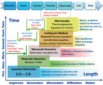
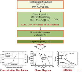

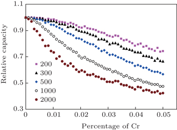
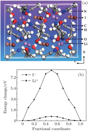

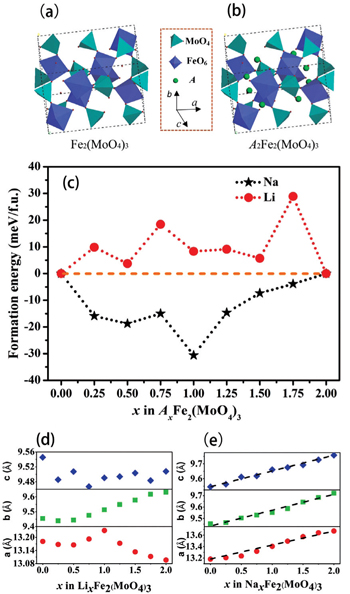
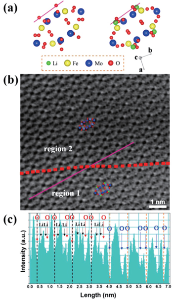

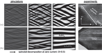
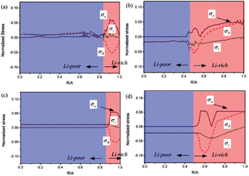
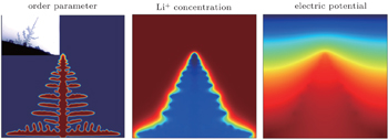


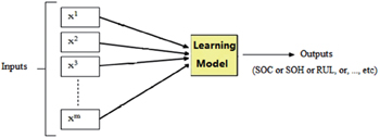

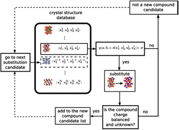

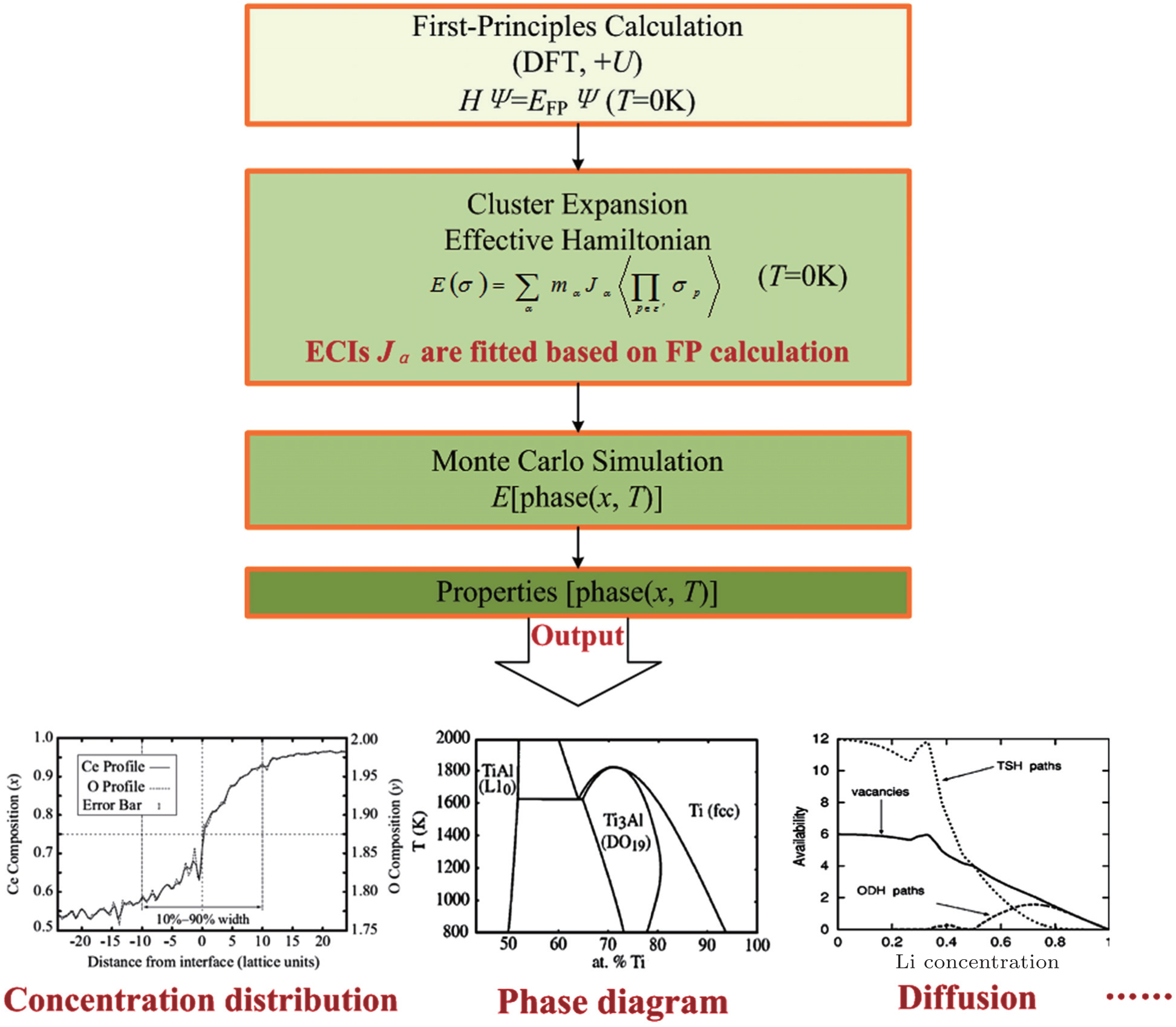
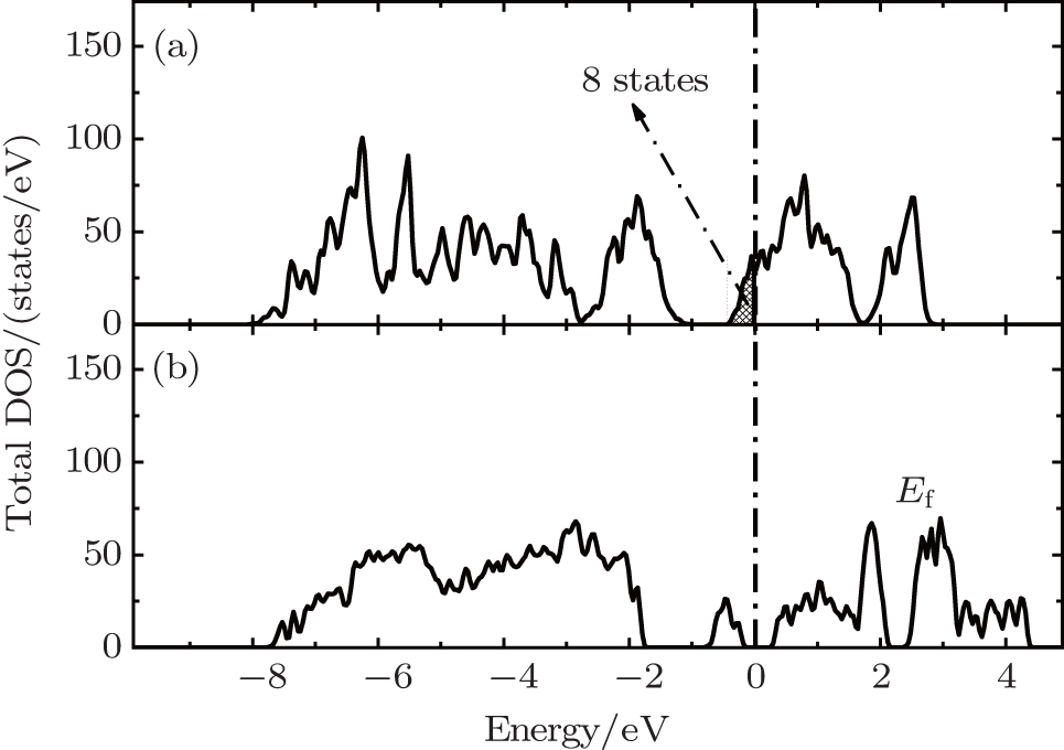
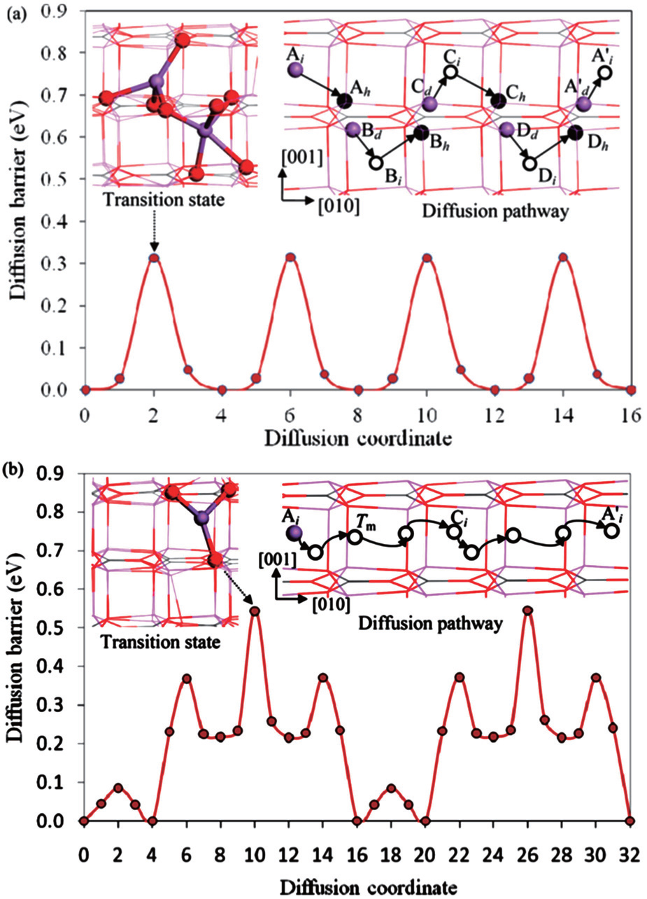


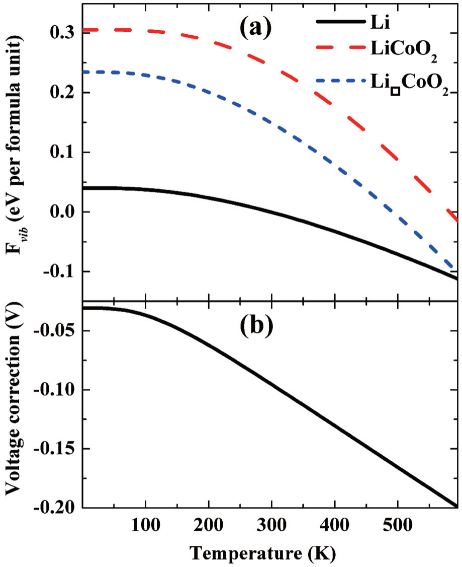

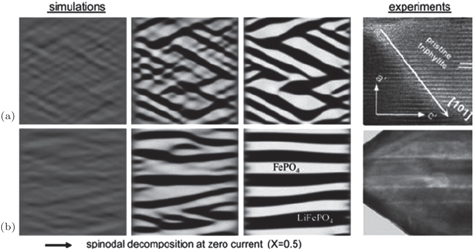

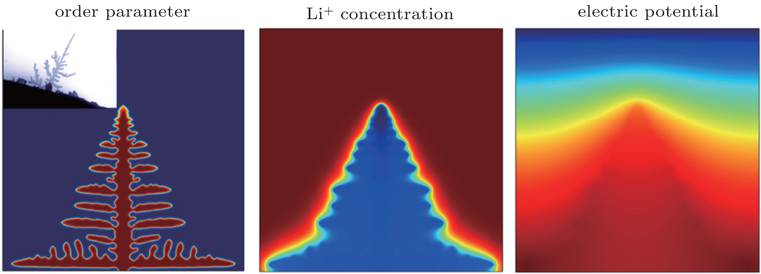
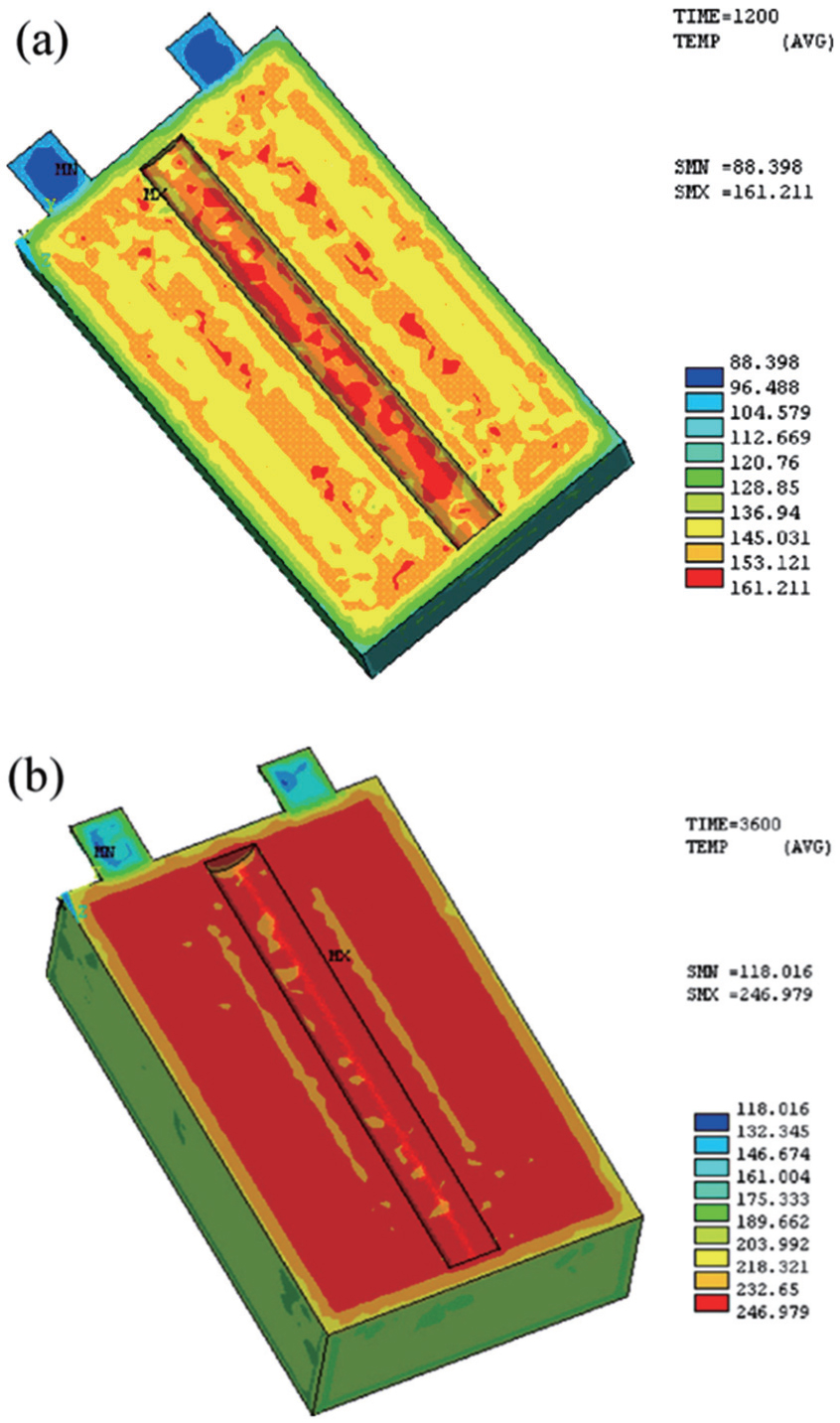
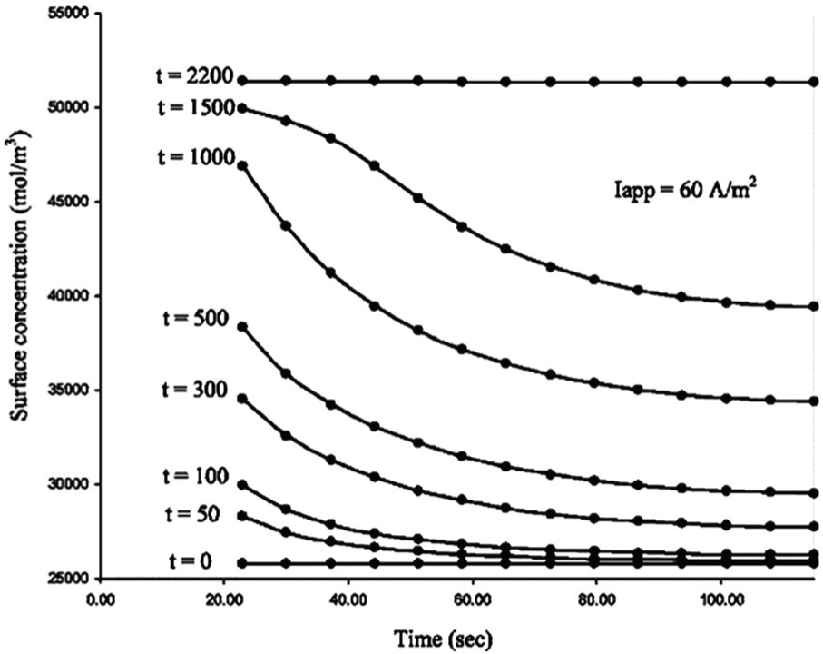
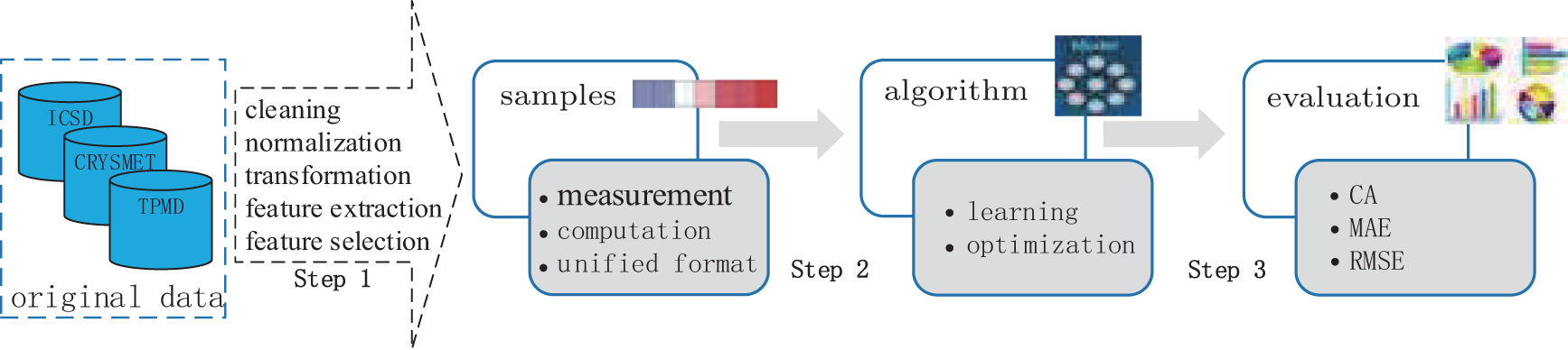
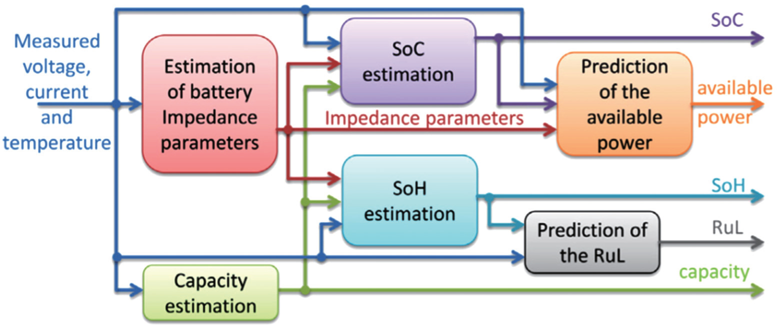
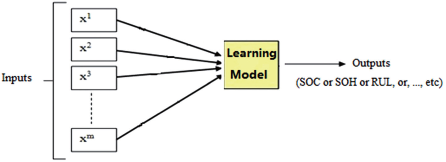
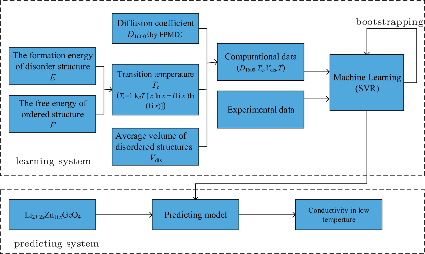

 , Gao Jian 2 , Liu Yue 3, ‡,