New developments in the multiscale hybrid energy density computational method
Sun Min 1 , Wang Shanying 2 , Wang Dianwu 1 , Wang Chongyu 1, 2, †,
Central Iron and Steel Research Institute, Beijing 100081, China
Department of Physics, Tsinghua University, Beijing 100084, China


† Corresponding author. E-mail: cywang@mail.tsinghua.edu.cn

Project supported by the National Basic Research Program of China (Grant No. 2011CB606402) and the National Natural Science Foundation of China (Grant No. 51071091).

Abstract
Abstract

Further developments in the hybrid multiscale energy density method are proposed on the basis of our previous papers. The key points are as follows. (i) The theoretical method for the determination of the weight parameter in the energy coupling equation of transition region in multiscale model is given via constructing underdetermined equations. (ii) By applying the developed mathematical method, the weight parameters have been given and used to treat some problems in homogeneous charge density systems, which are directly related with multiscale science. (iii) A theoretical algorithm has also been presented for treating non-homogeneous systems of charge density. The key to the theoretical computational methods is the decomposition of the electrostatic energy in the total energy of density functional theory for probing the spanning characteristic at atomic scale, layer by layer, by which the choice of chemical elements and the defect complex effect can be understood deeply. (iv) The numerical computational program and design have also been presented.

1. Introduction

The key problem in multiscale science is how to construct the model and to present the algorithm, both of which are involved in the physical connotation and the computational technique, as well as the related challenging problems — particularly for complex materials systems, including structural defects and chemical doping. A schematic pattern of multiscale is shown in Fig.  1 . [ 1 ]

Fig. 1. Multiscale of length and time.

To exploit the physics spanning multiscale and multilevel, the development of new approaches is required, which should overstep the sequential multiscale model that suits the multiscale weakly coupling systems, [ 2 4 ] while the multiscale correlation in a not-too-weak coupling system must be studied using the unifying model, based on, for examples, quantum mechanics (QM), molecular dynamics (MD), and finite elements (FM) methods. In order to treat the problem, the hybrid scheme is presented to drive progress, some examples are given in the reference papers. [ 5 10 ] One of the characteristics of the hybrid multiscale methods lies in coupling between quantum mechanics and molecular mechanics, some related papers have been published, [ 7 9 ] which have important scientific significance and application potential.

Considering the multiscale requirement of the physical connotation and the mathematical treatment method, the hybrid energy density method published [ 11 15 ] must be developed further. In the present paper, we first focus on the study to obtaining the coupling weight parameter in the energy coupling equation of the multiscale transition region. The second study is to decompose the non-homogeneous charge density into the lattice sites in the complex physical system according to the structural characteristics. In order to solve these problems, new physical thought and new computational method will be introduced. Then the total energy of the complex physical system should be expressed in the form of the sum of the site energies.

2. Physical basis of the developed multiscale hybrid energy density method
2.1. Representation of energy based on the theory of quantum mechanics of solids

The total energy can be expressed as the sum of the band energy and the electrostatic term, the expressions are written as follows: [ 11 , 16 , 17 ]

where E T is total energy of the studied system, E band is the band energy, E es [ ρ ( r )] is the electrostatic energy, E n is the eigenvalue, E l is the structural energy, Z is the atomic number, R l is the atom position, ρ ( r ) is the charge density, E xc is the exchange–correlation energy, and n αl is the partial density of state.

Equation ( 4 ) is the core formulation in our energy density method within density functional theory (DFT); the structural energy E l is closely related to the energy of the system studied.

2.2. Construction of the energy coupling expression in multiscale transition region

A theoretical model is presented for treating the coupling between the electronic effect of the local region and the classical influence of the long range environment. The weighting coupling energy expression in the transition region has been represented [ 11 , 12 ] by the site energy as follows:

where TR denotes the transition region, ω l is the coupling weight on site, is the site energy by DFT, is the site energy by MD, and the equivalence of the physical connotation for and is considered. [ 12 ] Because the binding energy is the basis for calculating the site energy by QM and by MD. From this consideration, the expression can be written as follows:

where is the binding energy of the studied system obtained by DFT, and is the energy of free atom.

Then we can define an expression as follows:

Equation ( 7 ) is suited for studying the characteristics of the site energy in the nonhomogeneous charge density system and for studying the homogeneous charge density system. The site energy of the electrostatic term for the homogeneous system of charge density can be written as where N is the total number of atoms.

2.3. Introducing and evaluating the weighting parameter ( ω ) in the transition region

The expression of energy coupling with weighting parameters of the entire system is constructed by site energy as follows:

where the weighting parameters and represent the contributions of the site energies respectively on each atomic position in the TR region. On the l -th site of the TR region, and obey constraint condition

In the present work, in order to obtain ω l ( l ∈ TR), the improvement for evaluating ω l is presented, we will compute ω l ( l ∈ TR) through an underdetermined system of linear equations.

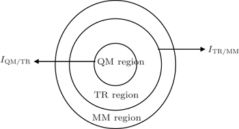
As shown schematically in Fig.  2 , here I QM/TR and I TR/MM denote the interfaces between different regions, and the subscripts signify the related regions. The constraint conditions are at the interface I QM/TR , and at the interface I TR/MM . These are used to guarantee the consistency of the physical quantities at the interfaces.

Fig. 2. Schematic representation of a spatially partitioned system which contains three regions. There are two interfaces: I QM/TR between regions QM and TR, and I TR/MM between regions TR and MM.

The energy of regions QM and TR (QM − TR) obtained by EDM should be equal to that calculated by using the DFT approach. The concrete energy coupling equation is expressed as

In the paper, we assume that ω l ( l ∈ TR) is invariant with the strain ranging from − ε to + ε in the calculated system, corresponding to a constraint equation. We formulate the problem of solving ω l ( l ∈ TR) as underdetermined linear equations of the system

Constraint conditions are as follows:

The Monte Carlo method is adopted to solve the underdetermined linear equations and seek the nonnegative ω l ( l ∈ TR). This is a major improvement from the previous EDM work, [ 11 , 12 ] as instead of using the empirical or the semi-empirical functions to fit the coupling parameters, we could get ω l ( l ∈ TR) by solving the underdetermined equations formulated by the given constraint conditions.

2.4. Ionic forces and dynamical relaxations

In the EDM, the forces are calculated by differentiating Eq. ( 8 ). For the l -th site in the QM region, the ionic force is computed as

where are the Cartesian coordinates of atom l in the QM region. By inserting the constraint condition ( l ∈ TR) into Eq. ( 12 ), we can obtain

where is the ionic force on the l -th atom when regions QM and TR are treated by the DFT method. Equation ( 13 ) can be written as [ 12 ]

The same can be applied to the MM region atoms, by which we can obtain

where is the m -th ionic force when regions MM and TR are treated with the MD method.

In the same way, the ionic force of the n -th site in the TR region can be computed as

From Eq. ( 16 ), which suits for the homogeneous system of charge density, we can see that the form of the EDM calculating the ionic force in the TR region is similar to the well-known linear force mixing method, which belongs to the force-based multiscale approaches.

The flowchart of the EDM is shown in Fig.  3 , illustrating the overall process of how the EDM works.

Fig. 3. Overall flowchart of the EDM.
3. Applications of EDM
3.1. Model and calculation method

The EDM is performed in a model that measures 35.2 Å × 35.2 Å × 105.6 Å with 12000 atoms in total. The x , y , and z axes correspond to [010], [001], and [100], respectively, and the periodic boundary conditions are applied in the x and y directions as shown in Fig.  4 . There are 60 (100) layers in the z direction in total. The atoms in each (100) plane have the same z coordinate and are equivalent to each other, so they share the same site energy and weighting parameter in the following calculations. The QM region includes the outermost seven (100) layers of the surface area (quantum mechanics area). And because of the equivalence of all the atoms in the same layer, the size of the QM region could be reduced to a 1 × 1 × 3 supercell, which measures 3.52 Å × 3.52 Å × 10.56 Å with 14 Ni atoms.

Fig. 4. Schematic diagram of the QM, TR ( n = 18), and MM regions.

Next, we will determine the critical dimension of the TR region. The dimension of the TR region should be large enough so that will not be affected by the atoms in the MM region and likewise will not be influenced by the surface area belonging to the QM region either. Besides, both the QM and TR regions are dealt with in DFT simulation, which demands a large TR region to avoid the influence of the interface TR/MM on region QM. However, as the size of the TR region increases, the DFT calculations can become computationally expensive. In this vein, we need to choose the proper magnitude of region TR to balance the desired accuracy and efficiency. We vary the size of the TR region as n layers in the z direction, in which n ranges from 2 to 32, with an interval of 2. In the above 16 different models, the position of the interface of TR/MM is at the 9th, 11th, 13th, …, 39th layer, respectively.

The DFT calculations are applied to both QM and TR regions with periodic boundary conditions in the x and y directions and a 12 Å vacuum layer in the z direction, as shown in Fig.  4 . The DFT calculations are carried out with the plane-wave based Vienna ab initio simulation package (VASP) [ 18 , 19 ] with the projector augmented wave pseudopotentials. [ 20 , 21 ] The Perdew–Burke–Ernzerhof generalized gradient approximation (PBE-GGA) [ 22 ] is employed. Plane waves have been included up to a cutoff energy of 350.5 eV for Ni. The k -point sampling is set up according to the Monkhorst–Pack scheme [ 23 ] with a 25 × 25 × 1 k mesh. The rest of the model belongs to region MM. The MM calculations are performed using the EAM potentials of Ni developed by Du et al. [ 24 ]

3.2. Correlation of the difference between and with the surface effect

In the TR region, atoms in the same (100) layer share the same site energy and weighting parameter ω l . is calculated in the above 16 models, and the results are shown in Fig.  5 . We can see that the behavior of of the 1st layer on the boundary tends to be smooth when n ≥ 18, which indicates that an 18-layer-measurement TR region can reflect the multiscale coupling characteristics. The size of the QM and TR regions needs to contain the 3.52 Å × 3.52 Å × 42.24 Å with 50 atoms in total.

Fig. 5. The calculated of the 1st layer in the 16 models, in which the number of layers n of the TR region ranges from 2 to 32.
3.3. and of the QM and TR regions

The and of each atomic site are calculated with n = 18. The results shown in Fig.  6 indicate that varies drastically in the topmost surface atomic layers and this behavior decays for about 11 layers into the bulk region. shows that the influence of the surface is only within the first three layers. So the site energy can be viewed as an energetic characteristic of the lattice structure and could represent the interesting quantum effect of the atomic site. The site energy and ionic force calculated by the DFT method at the interface TR/MM may be influenced by the vacuum layer; however, according to the boundary conditions brought up earlier, is zero at the interface TR/MM, which means that the inaccurate DFT site energy and force shall have no contributions to the binding energy and the ionic force according to Eqs. ( 9 ) and ( 16 ).

Fig. 6. and of the QM and TR regions along the z [100] direction with n = 18.
3.4. The weighting parameters

Based on the solution of the underdetermined equation, the weighting parameters are plotted in Fig.  7 . The number of each (100) layer in the TR region is denoted in Fig.  4 . The weighting parameters could represent the contributions of the two different methods at each atomic site in the TR region. The results show that for the first 14 layers in the TR region, the quantum mechanical effect plays a dominant role, while for the last four layers, this effect decays and the influence of the molecular dynamical simulation prevails.

Fig. 7. ω l of the atomic sites of each (100) layer in the TR region.
3.5. Distribution of charge density in the Ni system by DFT

The charge density of the EDM relaxed structure is calculated, and the results are plotted in Fig.  8 . The plane here corresponding to the xz plane of the model is shown in Fig.  4 . This data manifests that the quantum effect of the surface gradually vanishes from QM to TR region. This set of ω l ( l ∈ TR) must be used in Eq. ( 16 ) to represent and then the final ionic forces in the TR region can be given.

Fig. 8. The charge density on the (100) plane of the EDM relaxed structure. Positive (negative) values denote charge accumulation (depletion).
4. Development of the theoretical computational method for the non-homogeneity of charge density in a complex system

The key to the development of this theoretical algorithm lies in the decomposition of the electrostatic energy of the system into each atomic site, which can be predicted to realize the spanning scale correlation at the atomic scale layer-by-layer with the site energy; [ 11 , 13 ] then the information relevant to the choice of chemical elements and the control of defects may be provided for the problem of the electron behavior on atomic scale in the multiscale problems.

4.1. Decomposition of electrostatic energy of a system

The Kohn–Sham equation based on local spin density approximation (LSDA) can be represented as

where ∇ 2 is the Laplace operator, V ne ( r ) is the nucleus–electron potential, V ee ( r ) is the electron–electron Coulomb potential, is the exchange–correlation potential, Ψ ( r ) is the wave function, ρ ( r ) is the charge density, ε xc ( ρ , ξ ) is the exchange–correlation potential of free electron gas, η is the molecular orbital occupation number, and σ labels the electron spin ( σ = +, −).

The ground state energy of the system is given by using Born–Oppenheimer approximation within the framework of density functional theory

where T s [ ρ ( r )] is the kinetic term, which can be obtained from the Kohn–Sham equation based on local spin density approximation, E ee [ ρ ( r )] is the electron–electron Coulomb energy, E ne [ ρ ( r )] is the electron–nucleus attraction energy, E xc [ ρ ( r )] is the exchange–correlation energy, and E nn is the nucleus–nucleus repulsion energy.

Based on the analytic expression of the total energy of the computational system and the design of the numerical calculation program, we introduce a new parameter and define

Then the total energy of the system can be rewritten as

Equation ( 31 ) can be expressed as the sum of the band energy ( E band ) and the electrostatic energy ( E es [ ρ ( r )]). [ 16 ] Then the total energy of the calculated system can be expressed as

where

Considering Eq. ( 34 ), the total energy can be presented as

Based on the discrete variational method, [ 25 ] we can express an arbitrary 3D integration of multi-center function in the form of a weight summation of 3D quasi-random points

where i is the discrete variational point, f ( r ) is the multi-center function, and ω ( r i ) is the integration weight.

In order to realize the decomposition of the electrostatic energy of the system into each atomic site, it is necessary to partition 3D quasi-random points on each atomic region according to a Wigner–Seitz-like cell, and then correspondingly, the Coulomb energy and exchange–correlation energy will be partitioned on each atomic site, so that the total energy of the system can be written as

4.2. Numerical computational method for the decomposition of electrostatic energy

We adopt an efficient 3D integration method called Diophantine method proposed by Ellis [ 26 , 27 ] to calculate the electrostatic energy, where the integration of the electrostatic energy density within each Wigner–Seitz-like cell determines the part partitioned to each atom. The idea of the Diophantine method is using a weight summation of 3D quasi-random points to calculate the integration of the multi-center function. Considering the intense (smooth) variation of the electrostatic energy in the region close to (away from) the nucleus, especially the singularity at the nucleus, the 3D sample points are mostly concentrated in the region close to the nucleus. A distribution function D ( r ), which is the linear combination of Fermi-like function d v ( r ) centered in nucleus, is constructed to ensure the above consideration

where t ν is a weight parameter of nucleus v , and Σ ν t ν = 1; the Fermi decay factor β ν in general is chosen as 1.0, is the Fermi radius, and A ν is a normalization constant and determined by ∫ d ν ( r )d 3 r = 1.

The integration weight ω ( r i ) (in Eq. ( 38 )) of sample point i can be properly adopted as

where N is the total number of sample points. Based on the above analysis, the electrostatic energy can be expressed as

In our work, the numerical calculated program of the electrostatic energy of the system is presented; the computational flow is laid out in Fig.  9 . The algorithm of the decomposition of the electrostatic energy will be applied to study the electronic structure of superalloys.

Fig. 9. DV-DAC major flow chart. Here, is the matrix element of Hamiltonian of subsystem, is the basis function of subsystem, H α is the Hamiltonian of subsystem, C α is the combination coefficient of basis function in subsystem, is the eigenvalue of subsystem, β = 1/ κ B T , κ B is the Boltzmann constant, and α in expression is the mixing coefficient.
5. Summary

The development of theoretical computational methods has been proposed for treating the non-homogeneity of charge density systems with multi-alloying elements and a defect complex. We constructed the underdetermined equations for solving the weight parameters in the transition region of the energy coupling equation of the multiscale model and successfully used the equations to study the system of the homogeneous distribution of charge density. The theoretical algorithm for decomposing the electrostatic energy in the total energy of DFT into site energy has been proposed. The numerical computational program has been written.

Reference
1 Babcock W 2001 MaterialEASE 14: Computational Materials Science: A Primer (AMPTIAC)
2 Clementi E 1988 Philos Trans R. Soc. London A 326 445
3 Wang C Y Liu S Y Han L G 1990 Phys. Rev. B 41 1359
4 Wang C Y Liu S Y Han L G 1996 Defect Dissusion Forum 73 134
5 Abraham F F Broughton J Q Bernstein N et al. 1998 Comput. Phys. Commun. 12 538
6 Broughton J Q Abraham F F 1998 Phys. Rev. B 60 2391
7 Choly N Lu G Weinan E Kaxiras E 2005 Phys. Rev. B 71 094101
8 Eichinger M Tavan P Hutter J Parrinello M 1999 J. Chem. Phys. 110 10452
9 Ogata S Belkada R 2004 Comput. Mater. Sci. 30 189
10 Zhang S L Mielke S L Khare R Troya D Ruoff R S Schatz G C 2005 Phys. Rev. B 71 15403
11 Wang C Y Zhang X 2006 Current Opinion in Solid State and Materials Science 10 2
12 Zhang X Wang C Y 2008 Eur. Phys. J. B 65 515
13 Wang C Y 2004 Complex Syst. Complex Sci. 1 9 (in Chinese)
14 Wang C Y 2004 Multi-scale Modeling and Related Approaches The 3rd Japan–China Symposium on Computer Aided Materials and Molecular Design-crossover Challenges Science on Prediction and for Proactive Engineering October 24–26, 2004 Tokyo, Japan
15 Li Z Wang C Y Zhang X Ke S H Yang W T 2008 J. Phys.: Condens. Matter 20 345225
16 Volker Heine 1980 New York Academic Press 35 92 10.1016/S0081-1947(08)60503-2
17 Gyorffy B Pickett W 1977 Superconductivity in d and f Band Metals: Report of Rochester Conference Douglas D New York Am. Inst. Phys 10.1007/978-1-4615-8795-8
18 Kresse G Hafner J 1993 Phys. Rev. B 47 558
19 Kresse G Furthmüller J 1996 Phys. Rev. B 54 11169
20 Blöchl P E 1994 Phys. Rev. B 50 17953
21 Kresse G Joubert D 1999 Phys. Rev. B 59 1758
22 Perdew J P Burke K Ernzerhof M 1996 Phys. Rev. Lett. 77 3865
23 Monkhorst H J Pack J D 1976 Phys. Rev. B 13 5188
24 Du J P Wang C Y Yu T 2013 Modell. Simul. Mater. Sci. Eng. 21 015007
25 Ellis D E Painter G S 1970 Phys. Rev. B 2 2887
26 Ellis D E Benesh G A Byrom 1979 Phys. Rev. B 20 1198
27 Ellis D E 1981 Actinides in Perspective. Proceedings of the Actinides-1981 Conference 10–15 September 1981 Pacific Grove, California USA