Quantum key distribution (QKD) ^{[ 1 , 2 ]} allows two legitimate parties, Alice and Bob, to establish a common and secret key when the channel is accessible to an eavesdropper, Eve. Since the best-known Bennett–Brassard 1984 (BB84) protocol ^{[ 1 ]} was put forward, QKD has attracted more and more attention all over the world, due to its unconditional security based on the fundamental laws of physics: no-cloning theorem and the uncertainty principle. ^{[ 3 ]}

QKD has been developed well both theoretically and experimentally ^{[ 4 – 11 ]} in recent years. However, people have come across all sorts of difficulties in a real situation. ^{[ 12 ]} Though an ideal QKD system is unconditional security, in fact the necessary assumptions that ideal QKD system need are not easy to be satisfied. These practical factors such as finite resources and imperfections of setups, will undoubtedly threaten the security of the real QKD system, and Eve can take advantage of the leaks to attack the system. To prevent the attacks, many countermeasures have been applied. One of them is to employ the decoy-state method ^{[ 13 – 17 ]} which introduces two or more decoy states to confuse Eve so that she cannot distinguish the signal state from the decoy states. Another important approach is the notion of device-independent QKD (DI-QKD). ^{[ 18 – 28 ]} What is more, people make works to characterize the effects of the real imperfect factors on the security of QKD system in a mathematical way to give a security proof. ^{[ 12 ]}

The finite-length key is an important practical factor which needs to be solved in a real QKD system. Under ideal conditions, the data transformed between Alice and Bob are infinite, and QKD can generate the final secure key from the infinite data. However, in practice, the data above cannot be infinite. It may cause statistical fluctuations on relating parameters. When we regard the finite-length keys, we should reconsider the security bound in the asymptotic regime.

In recent years, many significant advances have been achieved. ^{[ 29 – 32 ]} In 2008, Scarani and Renner ^{[ 33 ]} creatively presented the smooth min-entropy theory to obtain the security bound for practical BB84 with finite-length keys. Then Tan and Cai ^{[ 34 , 35 ]} studied the passive decoy-state with finite-length keys and demonstrated its unconditional security. Their works show that the practical decoy state can reach the asymptotic limit, where the resource is large enough but not infinite. In 2014, Zhou et al. ^{[ 36 ]} presented a concise and stringent formula to calculate the key generation rate for QKD using SPDCSs with finite-length keys.

In this paper, we first briefly introduce the decoy state protocol. We focus on the passive decoy-state protocol and the differences from the active decoy-state protocol. Then we introduce the phase-randomized WCP source used for the passive decoy-state method. With this source, we describe the passive decoy-state protocol without considering the finite-length key.

The rest of this paper is organized as follows. In Sections 2 and 3, we briefly introduce decoy state protocol and the WCP source which has been transformed for the passive decoy-state method, respectively. Next, in Section 4, we consider the passive decoy-state method with the infinite-length key. The affect of the finite-length key on the passive decoy-state method is analyzed in detail in Section 5. The numerical simulations of this section are shown in Section 6. Finally, Section 7 concludes the paper with a summary.

In Section 1, we presented the fact that the necessary assumptions an ideal QKD system needs are not easy to satisfy. In the original proposal of the BB84 protocol, a single-photon source is necessary, but the single-photon source is still unavailable with current technology. Usually, a weak coherent pulse (WCP) source is used instead and many WCP-based experiments have been done since the first QKD experiment was carried out. ^{[ 37 ]} However, due to the multiphoton pulse sent from the WCP source, the QKD system will suffer from photon-number splitting (PNS) attack. ^{[ 38 , 39 ]} To protect the QKD system from PNS attack, one can use the decoy-state method which could closely reach the performance of single-photon sources. Actually, the method that Alice prepares the decoy state actively can be called the active decoy-state method. Similarly, the active decoy-state method also suffers from some practical factors. Because of imperfect experiments and channels, it may bring in some side channel information that Eve can take advantage of having an attack. For the real active (regular) decoy-state experiments, it is more difficult to verify the assumption that Eve cannot distinguish decoy and signal states. ^{[ 40 ]}

However, the passive decoy-state method ^{[ 41 , 42 ]} can reduce the side channel information in the decoy-state preparation procedure. Different from the active decoy-state method which actively changes the intensity of the laser pulses randomly, the passive decoy-state method only has one intensity pulse. The key point to distinguish in the passive decoy-state method is clicking or no clicking for Alice’s detector.

The common point between the passive decoy state and the active decoy state is that the yields and the error rates of the same photon-number states of the signal states and the decoy states shall be equal to each other, which means ^{[ 14 ]}

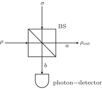
Due to the characters of the WCP source itself, it cannot be used for the passive decoy-state method directly. Curty et al. ^{[ 43 , 44 ]} have adjusted the WCP source to make it output two Fock diagonal states, so that it can be used for the passive decoy-state method. The fundamental setups are shown in Fig.  1 .

Fig. 1.

	Figure Option View Download New Window
	Fig. 1. The WCP sources [ 43 , 44 ] used for passive decoy-state method.

In Fig.  1 , ρ and σ denote the coherent states of two phase-randomized WCP source states, respectively,

Whenever the sender, Alice, does not care about the result of the measurement in mode b , the probability of having n photons in mode a can be written as

For Alice’s detector, the joint probability of having n photons in mode a and no click in the threshold detector now has the form

In this paper, we define that c denotes “click” of the detector while c̄ denotes “no click”. We also denote the signals that cause a click of Alice’s detector as signal states. The ones that cause no click of Alice’s detector are decoy states.

In this section, we discuss the ideal passive decoy-state method. In the passive decoy-state method, two-mode states are a prerequisite as shown in Fig.  1 . When Alice measures mode b with a threshold detector described by detection efficiency η _A and dark-count rate d _A , the mode a can be divided into two parts according to the result of the threshold detector: the “click” events and “no click” events. Here, we denote that the “click” events are signal states. The “no click” events are decoy states.

In Section 3, we have mentioned the parameter the probability of having n photons in mode a . It is divided into two parts and Usually, we describe as ^{[ 38 ]} Here, the parameters and can be written as

According to the passive decoy-state method, the counting rates and the error rates of the n -photon states of the signal states and the decoy states are

From Eqs. ( 10 ) and ( 11 ), it is easy to find that and have a relation. ^{[ 37 ]} In this paper, we use a parameter δ _n to represent it, that is

The overall gain of Alice’s detector producing a click is Q _c and no click is Q _c̄ . They can be expressed by

In order to calculate the lower bound of Q _{1, c̄} , we eliminate and elements. Applying equation (12) and the monotonicity of δ _n , we can obtain

Next, we will calculate the upper bound of error rates of the signal state and the decoy state. According to the quantum bit error rate (QBER),

Finally, taking the parameters above into the GLLP formula, one can obtain the following final key rate: ^{[ 42 ]}

Because of the finite-size data sets in real-life condition, parameters have various fluctuations. In this paper, we mainly consider the influence of the finite-size data on the single-photon yield and single-photon error rate. Here, we will use smooth min-entropy to study the passive decoy-state method with the finite-length key.

Firstly, we introduce some related definitions.

Compassable security definition ^{[ 45 , 46 ]} Assume a QKD protocol output keys of K _A and K _B on Alice’s and Bob’s sides, respectively. It is considered to be ε -secure if it satisfies both the correctness and the secrecy. Correctness means that the probability of K _A ≠ K _B will not exceed ε _cor , i.e.,

For QKD protocol, correctness can be regarded as the maximal probability of error-correction failure. Secrecy implies the probability that the final key is equal to the key without Eve is no less than 1 – ε _sec .

Smooth min-entropy ^{[ 45 ]} Let ε ≥ 0, σ _B ∈ S ( H _B ), and ρ _AB ∈ S _≤ ( H _AB ). The smooth min-entropy taken over a set of state B ^ε ( ρ ) that are ε -close to ρ _AB , is defined as

Chain-rule inequality for the smooth min-entropy ^{[ 47 ]} Let ε ≥ 0, ε ′, ε ″ ≥ 0, and ρ _ABC ∈ S _∈ ( H _ABC ), and then

Lemma 1 ^{[ 48 , 49 ]} Let ε _n , n _c , n _c̄ > 0, and let and be the quantum states of the “click” and “no click” n -photon events, respectively. They are both permutation-invariant quantum states, and let 𝔍 be a positive-operator-value measure (POVM) on H _AB which outputs the yield and quantum bit error rate, where Let ϒ _{n , c} and ϒ _{n , c̄} be the frequency distributions of the measurement events, e.g., the yield, when applying the measurements 𝔍 ^{n ₁} and 𝔍 ^{n ₂} , respectively. Then, for any elements Y _{n , c} and Y _{n , c̄} from ϒ _{n , c} and ϒ _{n , c̄} except with probability ε _n ,

Lemma 2 (Secret key based on smooth min-entropy) ^{[ 45 , 50 ]} By applying privacy amplification with two-universal hashing, a secret key extracted from X _A is ε _sec -secret if its length ℓ is chosen such that

Due to the influence of the finite-length key, the yields of the signal state and decoy state are no longer equal to each other, that is

Next, we can calculate the lower bound of the single-photon counting rates for the decoy state and signal state.

Similar to that in Section 4, we need to eliminate the elements of n ≥ 2 in Eq. ( 15 ). According to Eq. ( 30 ), the elements can be expressed by

Similarly, we can obtain the lower bound of Q _{1, c} according to inequalities ( 30 ), ( 37 ) and Eq. ( 14 ) as

Next, we will recalculate the upper bounds of e _{1, c} and e _{1, c̄} .

Due to e _{1, c} ≠ e _{1, c̄} , we can obtain two sample upper bounds of e _{1, c} and e _{1, c̄} from Eqs. ( 19 ) and ( 20 ), respectively,

To calculate the final key generation rate, Lemma 2 is usually used to obtain the length of the secret key firstly. In this paper, we set

Combined with the lower bounds of Q _{1, c} , Q _{1, c̄} and the upper bounds of e _{1, c} , e _{1, c̄} , equation (45) can be expressed by

According to the definition of the key generation rate, it is the fraction of the length of secret key and the number of total pulses, i.e., R = ℓ / N . One can obtain the final key generation rate as

However, it has been noted that the decoy state also has contributions to the key generation rate in the passive decoy-state method, so equation (44) is not suitable here. Recently, reference [ 36 ] considered the key generation rate of the decoy state of the passive decoy-state method and gave the length of the secret key in this situation as

The final secret key can be said to be ε _sec -secret if its length ℓ _{c + c̄} is chosen by

Now, combined with the lower bounds of the single-photon counting rate and the upper bounds of the error rate that have been calculated above, one can obtain the length of the final secret key as

According to the definition of the key generation rate, the final key generation rate under this condition is

Finally, the length of the final secret key is

In this section, we will take some numerical simulations to show how the finite-length key influences the final key generation rate of the passive decoy-state method. In the scenario we considered, the yields Y _n can be expressed by

The parameters , , and are calculated by Eqs. ( 6 )–( 8 ), respectively. We set μ _{1 = 0.5} and μ _{2 = 0.0001} . In this paper, ε _sec and ε _cor are 10 ^–10 and 10 ^–12 , respectively. The other parameter values in detail are listed in Table  1 . ^{[ 50 ]}

Table 1.

Table 1.

Table 1. Experimental QKD parameters. . α /dB·km –1 η Bob e d Y 0 η d d A f ( E c ), f ( E c̄ ) 0.2 0.1 0.005 1.7 × 10 –6 0.5 3.2 × 10 –6 1.16

Table 1. Experimental QKD parameters. .

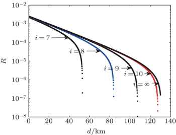
Figure  2 shows the relationship between the key generation rate R and the transmission distance d when the number N ( N = 10 ⁱ , i = 7, 8, 9, 10, ∞) of the total pulses from the WCP source is fixed by different values. From Fig.  2 , we can directly see that R becomes smaller with the increase of d . When the transmission distance d is fixed, the key generation rate R is getting larger with the increase of N . Meanwhile, when N is very small (e.g., N = 10 ⁷ ), the declining rate is fast. It would generate few keys if d ≥ 55 km. The curve of N = 10 ¹⁰ is getting close to the ideal situation; it indicates that the number of total pulses from the WCP source can really influence the QKD system. When the number of total pulses is larger than 10 ¹⁰ , the passive decoy-state QKD with the WCP source can implement well. However, by comparing these results with the results in Ref. [ 50 ], it can be seen that the passive decoy-state method is weaker than the active one both in the key generation rate and the extra transmission distance.

Fig. 2.

	Figure Option View Download New Window
	Fig. 2. Key generation rate R versus transmission distance d with different N ( N = 10 i , i = 7, 8, 9, 10, ∞).

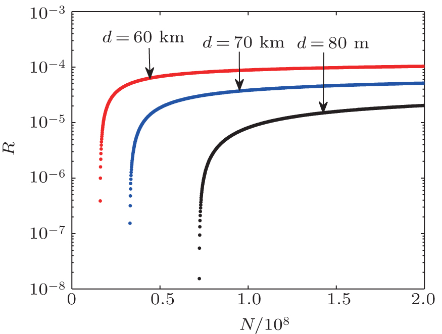
Figure  3 shows the relationship between the key generation rate R and the number of total pulses N when the transmission distances are different. We can find that the passive decoy-state method can generate keys when N is 2 × 10 ⁷ , 3.5 × 10 ⁷ , 7 × 10 ⁷ with 60 km, 70 km, and 80 km. When R is fixed, it needs more pulses with d becoming larger.

Fig. 3.

	Figure Option View Download New Window
	Fig. 3. Key generation rate R versus N with different d .

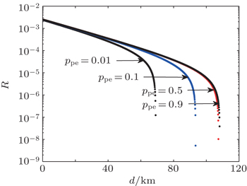
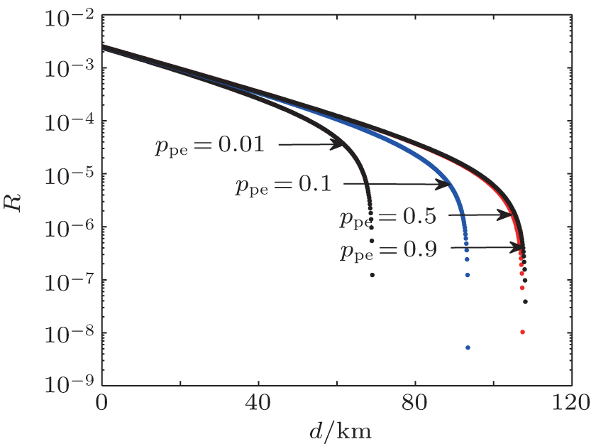
Finally, we analyse the relationship between R and d with different p _pe which means the probability of choosing a pulse as the sample bits used for parameter estimation when N is fixed. Figure  4 is an example whose N = 10 ⁹ . When the transmission distance is 60 km, it is easy to find that the lines of p _pe = 0.5 and p _pe > 0.5 are coincident which means that the key generation rates of p _pe = 0.5 and p _pe > 0.5 are almost equal. According to the definition of p _pe , the more pulses will be used to generate the key if it is getting smaller. Then, the QKD system can get more secure key bits. Hence, considering a compromised scheme, we take p _pe = 0.5 as an optimal reference value.

Fig. 4.

	Figure Option View Download New Window
	Fig. 4. Key generation rate R versus transmission distance d with different p pe .

In summary, we introduce the decoy state method and analyze the phase-randomized WCP source that can be used in passive decoy-state protocol. Then, we study the passive decoy-state method using the WCP source with an infinite-length key. After recalculating the phase error rate, counting rate, and error rate of the single photon state, we obtain the length of the secret key considering both the signal state and the decoy state in the passive decoy-state method. According to the results of numerical simulations, we find that the finite-length key influences the real QKD system. It can affect the key generation rate and the transmission distance. The key generation rate and the extreme transmission distance become larger with the increase of the number of total pulses. When the number is larger than 10 ¹⁰ , the passive decoy-state QKD with the WCP source will perform well. Meanwhile, we study the relationship between the key generation rate and the probability of choosing a pulse as the sample bits used for parameter estimation. It can help us to select the optimal value to make sure that the passive decoy-state method in this paper will be implemented best. Our work can help QKD experimentalists to improve the performance and provide references about how to choose the data-size.