†Corresponding author. E-mail: liuxian@ysu.edu.cn
*Project supported by the National Natural Science Foundation of China (Grant Nos. 61473245, 61004050, and 51207144).
Neural mass models can simulate the generation of electroencephalography (EEG) signals with different rhythms, and therefore the observation of the states of these models plays a significant role in brain research. The structure of neural mass models is special in that they can be expressed as Lurie systems. The developed techniques in Lurie system theory are applicable to these models. We here provide a new observer design method for neural mass models by transforming these models and the corresponding error systems into nonlinear systems with Lurie form. The purpose is to establish appropriate conditions which ensure the convergence of the estimation error. The effectiveness of the proposed method is illustrated by numerical simulations.
The electroencephalography (EEG) signal reflects the electrical activity of neurons within the cerebral cortex. It has been widely applied in brain research, [1, 2] especially in the diagnosis and therapy of neurological diseases, such as epilepsy, [3] schizophrenia, [4] and Parkinson’ s.[5] The mathematical modeling of EEG signals provides a powerful tool for mechanism analysis of neurological diseases.[6] Neural mass models are constructed from the perspective of the neural system structure and represent the mean activity of the whole neural population with lumped state variables.[7] They have been the preferred models to produce EEG signals since the 1970s[8] because they are very simple and have physiological meaning.[7] In recent years, different types of neural mass models have been developed to represent the generation of EEG signals with different rhythms, [7, 9] and they have been further used to examine the influence of coupling strength and propagation delay on specific rhythms.[10– 12] Meanwhile, a number of control strategies[13– 16] from control theory have been designed to adjust rhythms the produced by neural mass models.
State-feedback control is one of the most common strategies in control theory, which requires us to obtain all of the state variables to realize it.[17] However, it is difficult for a specific system, especially for the extremely complicated brain system, to derive all of the state information. The observer is able to reconstruct all of the states and plays an important role in the realization of state-feedback control[18, 19] and brain research.[20] Recently, observer design for neural mass models has been investigated by using absolute stability theory because these models can be represented as Lurie-type nonlinear systems.[21] The linear matrix inequality (LMI) method is used to solve the observer gain matrices in existing results.[22] The key problem in observer design is to guarantee the convergence of the estimation error and make the estimation error as small as possible. The results based on the circle criterion lead to infeasible LMI conditions which cannot ensure the convergence of the estimation error.[23– 25] Generalized results that lead to feasible LMIs are reported and cause the designed observer to be applied to the considered neural mass models.[26, 27] Our recent progress in the Lurie system theory to analyze and design time-delay nonlinear systems and complex dynamical networks has promoted us to use the developed techniques to analyze and design neural mass models.[28– 32] Here, we further improve the observer design method for neural mass models by using Lurie system theory and mathematical manipulation. The superiority of the proposed method is illustrated in the last section, which is devoted to numerical comparisons.
Notation The ℝ and ℝ n denote the set of real numbers and n-dimensional real column vectors, respectively. The notation I denotes an identity matrix with an appropriate dimension. A block diagonal matrix with square matrices Ai is denoted as diag(A1, … , An). The symmetric block component of a symmetric matrix is denoted by ⋆ . The vector norm is denoted by | · | . The L2 norm is denoted by ∥ · ∥ 2.
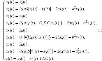
We consider the neural mass models with the dynamics described by eight first-order differential equations

where the variables x1, x3, x5, and x7 are the outputs of different types of postsynaptic potential blocks, x2, x4, x6, and x8 are the time derivatives of x1, x3, x5, and x7, respectively. The input p(t) is the afferent influence from neighbouring or more distant populations, and it is modeled by a Gaussian white noise with mean value 220 and standard deviation 30. The output z ∈ ℝ is the EEG measurement available to the observer, and ω ∈ ℝ is the measurement noise. The constants C1, C2, C3, and C4 are the average number of synaptic connection between pyramidal cell populations and interneuron populations; θ A and θ B are the average excitatory synaptic gain and the average inhibitory synaptic gain; a and b are the membrane average time constant and dendritic tree average time delays; ad is the average time delay on efferent connection from a population; and, D is a known number. The nonlinear sigmoid function S(· ) is of the form

When e0 = 2.5 s− 1, v0 = 6 mV, r = 0.56 mV− 1, the property of S(· ) is presented as Fig. 2. All of the values of the constants in the model are non-negative and their physiological meaning can be found in Ref. [9].
Observer design for Eq. (1) plays an important role in brain research.[20] There are many existing results relating to observer design for Eq. (1).[26, 27] The main purpose is to improve the observer design method and present less conservative conditions to achieve a smaller estimation error.
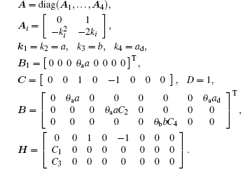
To realize the main purpose, we formulate Eq. (1) as a Lurie system

where

u is the input, and

Each entry of the state-dependent nonlinearity f (Hx) is a function of a linear combination of the states

where hl = [hl1 · · · hl8]. This satisfies a certain slope-restricted condition

where 

where x̂ is the estimation of state, d is the disturbance of input, K ∈ ℝ 3× 1 and L ∈ ℝ 8× 1 are the observer matrices to be designed. By defining the observer error as e = x̂ − x, we have

where φ (e, t) = f (V) − f (U), V = Hx̂ + K(Cx̂ − z), U = Hx. It follows from Eq. (5) that each entry of the nonlinearity φ (e, t) satisfies

Thus, the error dynamics (7) also have a standard form of Lurie system. The task of observer design for Eq. (3) is to design appropriate observer matrices K and L such that the observer error e satisfies

where scalars κ > 0, ρ d ≥ 0, and ρ ω ≥ 0. The designed observer is able to suppress the effect of input disturbance and measurement noise to a prescribed level ρ d and ρ ω if equation (9) is fulfilled. In order to keep the observer error as small as possible, ρ d and ρ ω need to be optimized.
In this section, we use the Lurie system theory and matrix manipulation to design the observer for Eq. (3) since the error dynamics possess a standard form of Lurie system.
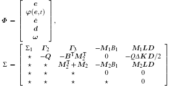
Theorem 1 If there exist a positive-definite matrix P = PT > 0, a positive semi-definite diagonal matrix Q ≥ 0, matrices K and L, free weighting matrices M1 and M2 with appropriate dimensions, scalar constants ɛ > 0, rω ≥ 0, rd ≥ 0, such that

then the observer error e satisfies Eq. (9), where
Proof Choose a Lyapunov functional candidate in the form of V (e) = eTPe, where P > 0. Calculating the time derivative of V (e) along the trajectory of the error dynamics (7) yields

Setting ql ≥ 0 (l = 1, 2, 3) and Q = diag(q1, q2, q3), it follows from Eq. (8) that


where φ (e, t) = [φ 1(e, t), φ 2(e, t), φ 3(e, t)]T. By combining Eq. (13) with Eq. (11), we have

Moreover, it follows from Eq. (7) that there exist any two matrices M1 and M2 such that

Combining Eq. (15) with Eq. (14) derives

where

and 
By applying Eq. (10), we obtain

When d = 0 and ω = 0, equation (16) reduces to V̇ (e) ≤ − ɛ eTe and consequently V̇ (e) is negative definite. This qualifies V(e) as a Lyapunov function. We demonstrate by the Lyapunov’ s stability theorem that the equilibrium e = 0 is asymptotically stable. When d ≠ 0 and ω ≠ 0, integrating Eq. (16) yields

Thus, we derive Eq. (9) with 

Theorem 1 provides a sufficient condition to keep the observer error e satisfying Eq. (9). The following optimization algorithm presents a way of deriving the minimum values of ρ d and ρ ω when ɛ is left unchanged:

We denote the minimum values of ρ d and ρ ω as ρ dmin and ρ ω min, respectively.
By setting M2 = α M1, formula (10) is turned into an LMI, and is able to be solved by using the LMI toolbox in MATLAB.
Theorem 2 If there exist a positive-definite matrix P = PT > 0, a positive semi-definite diagonal matrix Q ≥ 0, matrices Y1 and Y2, free weighting matrices M1 with appropriate dimensions, scalar constants α , ɛ > 0, rω ≥ 0, rd ≥ 0, such that

then 


Theorem 1 is simplified as follows when the input disturbance and measurement noise are not taken into account.
Theorem 3 Consider the plant (3) and the observer (6) with d = 0 and ω = 0. If there exist a positive-definite matrix P = PT > 0, a positive semi-definite diagonal matrix Q ≥ 0, matrices K and L, free weighting matrices M1 and M2, a scalar constant ɛ > 0, such that

then the origin of the observer error system (7) is globally asymptotically stable, where Γ 1, Γ 2, and Γ 3 are defined as Theorem 1.
In this section we will confirm the effectiveness of the designed observer and compare the proposed results with those in Refs. [26] and [27].
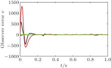
We consider the input disturbance d ∼ N(0, 0.12) and the measurement noise ω ∼ N(0, 0.92) in the design of observer. The system parameter D is set to D = 1. We solve the optimization problem (17) with the YALMIP toolbox in Matlab and derive ρ ω min = 434 and ρ dmin = 3.30. The time evolutions of the states x1– x8 of the neural mass model (black lines) and the states of the observer (6) obtained from Theorem 1 (red lines) are shown in Fig. 2. The time evolution of the observer error is shown in Fig. 3. We observe that the observer error nearly converges to zero, and the estimated states converge well to the states of the neural mass model. Keep the system parameters unchanged. We obtain ρ ω min = 706, ρ dmin = 9.48, ρ ω min = 596, and ρ dmin = 3.53, respectively, by using the methods given by Refs. [26] and [27]. This illustrates that the proposed method here is better than the existing results in Refs. [26] and [27].
We have presented a new observer design method for neural mass models by transforming both the models and the corresponding error systems into nonlinear systems with the Lurie form. The designed observer can suppresses input disturbance and measurement noise well. We have demonstrated the superiority of the proposed method by comparing it with some of the existing results. Although the method is put forward for neural mass models, it is applicable to other neural models or nonlinear systems with the specific structure of the Lurie form.
| 1 |
|
| 2 |
|
| 3 |
|
| 4 |
|
| 5 |
|
| 6 |
|
| 7 |
|
| 8 |
|
| 9 |
|
| 10 |
|
| 11 |
|
| 12 |
|
| 13 |
|
| 14 |
|
| 15 |
|
| 16 |
|
| 17 |
|
| 18 |
|
| 19 |
|
| 20 |
|
| 21 |
|
| 22 |
|
| 23 |
|
| 24 |
|
| 25 |
|
| 26 |
|
| 27 |
|
| 28 |
|
| 29 |
|
| 30 |
|
| 31 |
|
| 32 |
|


