


Establishment, maintenance, and re-establishment of the safe and efficient steady-following state
[Pan Deng† , Zheng Ying-Ping]
, Zheng Ying-Ping]
|
|


†Corresponding author. E-mail: pandeng@tongji.edu.cn
*Project supported by the National Natural Science Foundation of China (Grant No. 61174183).
We present an integrated mathematical model of vehicle-following control for the establishment, maintenance, and re-establishment of the previous or new safe and efficient steady-following state. The hyperbolic functions are introduced to establish the corresponding mathematical models, which can describe the behavioral adjustment of the following vehicle steered by a well-experienced driver under complex vehicle following situations. According to the proposed mathematical models, the control laws of the following vehicle adjusting its own behavior can be calculated for its moving in safety, efficiency, and smoothness (comfort). Simulation results show that the safe and efficient steady-following state can be well established, maintained, and re-established by its own smooth (comfortable) behavioral adjustment with the synchronous control of the following vehicle’s velocity, acceleration, and the actual following distance.
Safety and efficiency are very important for vehicle following control systems. In general, safe and efficient vehicle following movement should be realized by vehicle behavioral adjustment in smoothness (comfort). Pipes[1] brought forward a linear car-following model based on the presupposition of “ law of separation” , but “ a certain prescribed following distance” does not reflect the complexity and rapid change of vehicle following situation. It is hard for “ a certain prescribed following distance” to give considerations to both the safety and the efficiency of the following vehicle’ s behavioral adjustment all of the time. Dunbar and Caveney[2] presented a distributed receding horizon control algorithm for vehicle platoon control with the constant desired separation distance. Li et al.[3] proposed a good hierarchical control architecture model, in which it seems to be questionable that the stopping distance of typical truck is taken to 5 m all the time. Chandler et al.[4] found that the constant distance between vehicles at different speeds will lead to an unstable following state. Considering the lateral separation characteristics between the follower and the leader, a non-lane-based model of car following was developed by Jin et al.[5] on the basis of time-to-collision and the stimulus– response framework to enhance safety. Another famous model is the optimal velocity model presented by Bando et al.[6, 7] to describe many features of vehicle following operation. Unfortunately, the classical optimal velocity (OV) model locally oscillates with vehicles colliding and moving backward.[8] Helbing and Tilch[9] put forward a generalized force (GF) model which overcame some shortcomings of the OV model, but only considered the influence of vehicular behavior, given by the negative velocity difference. In order to avoid the deficiencies of the GF model, Jiang et al.[10] presented a full velocity difference (FVD) model which can simulate the phase transition in traffic flow and the evolution of traffic congestion. Aiming at the driving behavior, emergencies, and avoiding traffic collision and the impractical acceleration of the OV model, Zhao and Gao[11] built a full velocity and acceleration difference (FVAD) model, but there was a lack of clarity in the integration between the velocity difference control and the acceleration difference control. A new optimal velocity difference mode was established by Peng et al.[12] to avoid collision and eliminate the unrealistically high deceleration. The disadvantages are that the dynamic determination of the correlation coefficients in practical application has no effective, feasible, or general solution. In theory, the above research results in Refs. [9]– [12] can help vehicle following system establish a safe and efficient steady-following state, but how to in real time determine the coefficients of the mathematical models presented in Refs. [9]– [12] has been a problem, which restricts its engineering applications to a certain extent. In order to reduce the complexity of the models mentioned in Refs. [9]– [12], Tordeux and Seyfried[8] raised a new OV model with no additional parameters, which is intrinsically asymmetric and collision-free for any value of the inputs. Pan and Zheng[13] used the fitting function to calculate the dynamic safe following distance, by which the following vehicle’ s behavioral quality can be evaluated and controlled for safety, efficiency, and smoothness (comfort). Desjardins and Chaib-draa[14] used the function approximation techniques as a means of directly modifying a control policy to optimize the performance of vehicular cooperative adaptive cruise control system. The safety of vehicle following could be undoubtedly guaranteed but there were no further discussion and analyses given to the efficiency of vehicle following. In Ref. [15], for the safety, efficiency, and smoothness of vehicular adaptive cruise, Kesting et al. used the intelligent driver model[16] to represent adaptive cruise control (ACC) vehicles and presented an ACC strategy where the acceleration characteristic can automatically adapt to different traffic situations. However, there is a lack of clarity about how to calibrate the safe time gap scientifically in the dynamic traffic situation. Ge and Orosz[17] proposed a connected cruise control model with delayed acceleration feedback to increase roadway traffic mobility and robust performance. Obviously, vehicle following (adaptive cruise) control under vehicular networking technology has become a focus of study.
Energy saving is another hot area of study in vehicle following control. Tang et al.[18, 19] and Yang et al.[20, 21] established the energy consumption models of car-following systems. Simulation and experiments have shown that under the smooth driving behavior the electric vehicle’ s battery lifetime can be prolonged and energy consumption will increase with traffic interruption, accelerating or decelerating suddenly. The research results of Shi and Xue[22] showed that for a stabler traffic flow, the low energy consumption becomes lower. Nakayama et al.[23] pointed out that traffic congestion results in the consumption of much fuel and the change of velocity leads to the additional consumption of energy compared with the case of no disturbance. A conclusion can be drawn that for a stable vehicle following system, the following vehicle can move in safety, efficiency, and smoothness (comfort) at any time.
Many scholars and researchers, such as Newell, [24] Kerner, et al., [25– 32] Lee H Y, et al., [33] Lee H K, et al., [34] Tomer, et al., [35] Helbing, et al., [36] Nagatani, [37] Naito, et al., [38, 39] Sugiyama, et al., [40, 41] Lenz, et al., [42] Kurata, et al., [43] Jiang, et al., [44, 45] Ge, et al., [46, 47] Tang, et al., [48– 50] Peng, et al., [51] Yu, et al., [52– 54] Zhang, [55] Zhou, et al., [56] and Zhu et al.[57] have studied the stability and evolution of traffic flow with the influence of vehicle longitudinal and lateral behaviors from a point of view of statistical physics and nonlinear dynamics. Undoubtedly, it is of great advantage for us to have a profound understanding of internal rules of traffic flow and vehicle following movement. These hard-earned achievements will help us explore the control methods of vehicle following operation in smoothness (comfort) and the management schemes of traffic flow for energy saving. Kerner[58] showed a great insight into the generally accepted fundamentals and methodologies of traffic and transportation theory. His valuable and enlightened academic views will promote the future study of vehicle following operation and traffic flow.
The above research results laid the foundation for the further study of vehicle following (control) systems. However, vehicle following operation in safety, efficiency, and smoothness (comfort) is different from the establishment, maintenance, and re-establishment of the safe and efficient steady-following state. The latter can be realized by the former but vehicle behavioral adjustment in safety, efficiency, and smoothness (comfort) does not necessarily help the vehicle following system establish the safe and efficient steady-following state, including the previous safe and efficient steady-following state and the new one. We think that the purpose of vehicle following control is just to establish, maintain, and re-establish the safe and efficient steady-following state, in which two successive vehicles move at the same velocity and the actual following distance between them is a little greater than or equal to the safe following distance, not to change their own behaviors endlessly. In this paper, regarding the safe and efficient steady-following states as the optimization goals, we utilize the hyperbolic functions to establish the mathematical models for the engineering calculation of vehicle following behavior at any time, by which vehicle following system can move in safety, efficiency, and smoothness (comfort) under any following situation.
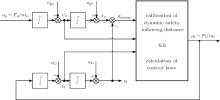
A block diagram of vehicle following control system is shown in Fig. 1. Here, ap and af are the accelerations of the preceding and following vehicles, respectively, Fp and Ff are the resultant traction force of the preceding and following vehicles, respectively, mp and mf are the mass of the preceding and following vehicles respectively, vp and vf are the velocities of the preceding and following vehicles respectively, sp and sf are the positions of the preceding and following vehicles, respectively, vp0 and vf0 are the initial velocities of the preceding and following vehicles, respectively, sp0 and sf0 are the initial positions of the preceding and following vehicles, respectively, dactual is the actual following distance of the following vehicle away from the preceding vehicle.
Suppose that dsafe is the safe following distance, which should be kept by the following vehicle from the preceding vehicle for safety and efficiency. On the other hand, the length of dactual based on dsafe has its effect on the smoothness (comfort) of the control strategies to be adopted by the following vehicle. It is clear that dsafe can be determined by the velocities and control strategies of the preceding and following vehicles. In every sampling period, the real-time calibration of dsafe can help us to understand the quality of the vehicle following operation in safety and efficiency, and determine an optimization target of vehicle following behavior.
 | Fig. 1. Block diagram of vehicle following control system. |
Let Δ v = vp − vf and Δ d = dactual − dsafe again. By the reasonable control laws, the following vehicle can adjust its own behavior to establish a safe and efficient steady-following state, in which ap = af = 0, Δ v = 0, and Δ d is a little greater than or equal to zero. In the process of the following vehicle adjusting its own behavior, the synchronous control of af, Δ v, and Δ d is the key to establishing the safe and efficient steady-following state. Due to the characteristics of the hyperbolic functions, we will use them to establish the corresponding mathematic models for the following vehicle to adjust its own behavior scientifically.
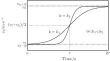
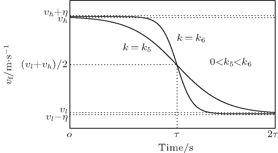
Figure 2 describes the whole accelerating process of the following vehicle from a velocity to another higher velocity.
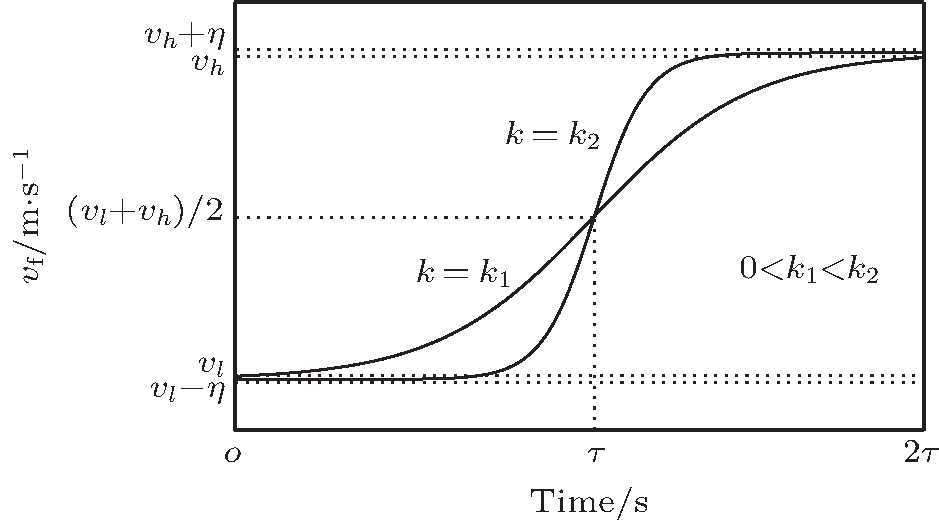 | Fig. 2. Accelerating from vl to vh (vl < vh). |
The corresponding mathematic model of the following vehicle speeding up can be expressed as follows:
where vf(t) denotes the velocity– time curve of the following vehicle accelerating from vl to vh, k is a coefficient greater than 0, τ is a positive time constant, and η is a small positive number for the convenience of the engineering calculation because the hyperbolic tangent function tanh(k(t − τ )) would infinitely approach − 1 or + 1, respectively, when t → − ∞ or t→ + ∞ , and in engineering we cannot accept this situation that too much time is spent by a vehicle on its own behavioral adjustment to establish the safe and efficient steady-following state. Clearly, parameter k is closely related to the rapidity and smoothness (comfort) of vehicle behavioral adjustment.
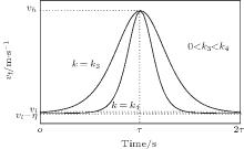
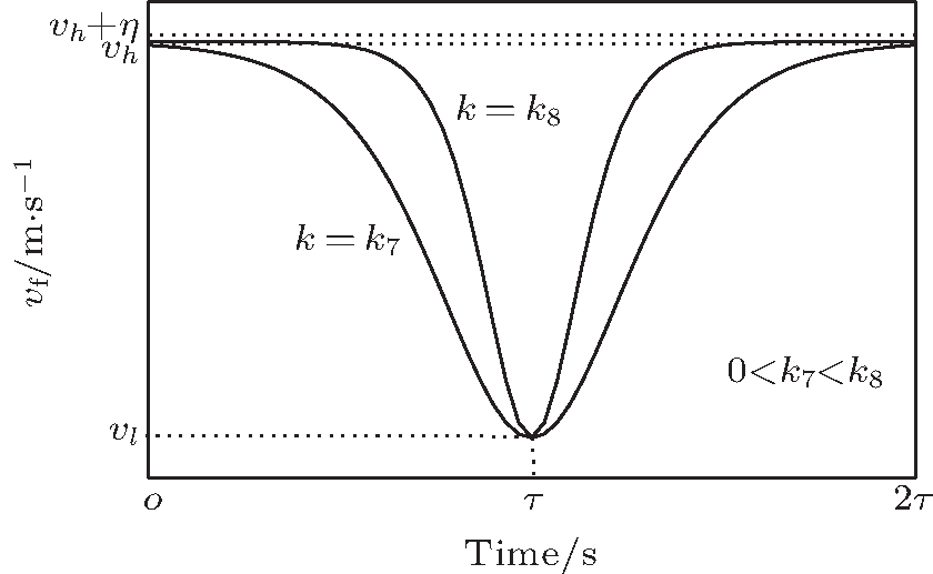
Figure 3 describes the whole process of the following vehicle first accelerating and then decelerating from vl to vh.
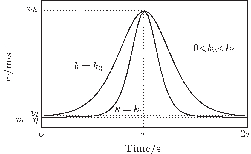 | Fig. 3. First accelerating and then decelerating from vl to vh. |
Here, vh denotes a maximum velocity value in the whole process of the following vehicle adjusting its own behavior. The corresponding mathematic model is shown as follows:
where parameter k is closely related to the rapidity and smoothness (comfort) of vehicle behavioral adjustment.
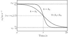
Figure 4 describes the whole decelerating process of the following vehicle form a velocity to another lower velocity.
 | Fig. 4. Decelerates from vh to vl (vl < vh). |
The behavioral change of the following vehicle can be described by the following mathematic model:

where parameter k is closely related to the rapidity and smoothness (comfort) of vehicle behavioral adjustment.
The curve of the following vehicle adjusting its own behavior in the manner of first decelerating and then accelerating from vh to vh is shown in Fig. 5.
 | Fig. 5. The following vehicle first accelerates and then decelerates from vh to vh. |
The corresponding mathematical model can be expressed as follows:

where parameter k is closely related to the rapidity and smoothness (comfort) of vehicle behavioral adjustment.
Clearly, by changing the values of k, τ , and η in Eqs. (1)– (4), we can obtain different accelerating and/or decelerating processes with their corresponding time-varied accelerations and traveling distances. In turn, according to the present following situation and the optimization objective of the following vehicle’ s behavior in safety, efficiency, and smoothness (comfort), we can determine the corresponding mathematical model to be used to calculate the control law for the behavioral adjustment of the following vehicle.
Equations (1)– (4) can be used by the following vehicle not only to adjust its own behavior for improving the safety or efficiency but also to help vehicle following system establish a previous or new safe and efficient steady-following state. The flexible application of Eqs. (1)– (4) can synchronously control the values of af, Δ v, and Δ d in the process of the following vehicle adjusting its own behavior. In addition, the behavioral adjustments of the following vehicle are expected to be also smooth or comfortable. References [59]– [62] have given the comfort (smoothness) standard of vehicle’ s behavioral adjustment. The reasonable values of k, τ , and η in Eqs. (1)– (4) can help the following vehicle move in safety, efficiency, and smoothness (comfort).
The control laws of the following vehicle adjusting its own behavior can be calculated by the algorithm shown in Fig. 6.
 | Fig. 6. Algorithm of the following vehicle adjusting its own behavior during every sampling period. |
In Fig. 6, vp0 and vf0 are, respectively, the velocities of the preceding and following vehicles at the initial time of the following vehicle adjusting its own behavior during every sampling period, dsafe0 and dactual0 are, respectively, the safe and actual following distance at this time.
The following vehicle should adjust its own behavior under the constraint of the traveling distance dactual0 − dsafe0 for efficiency improvement: if vf0 < vp0, the following vehicle will speed up according to Eq. (1) to establish a safe steady-following state. If vf0 = vp0, there is a safe steady-following state between two successive vehicles. Equation (2) will be used by the following vehicle to reduce the actual following distance to establish a safe and efficient steady-following state. If vf0 > vp0, the following vehicle will decelerate according to Eq. (3) to improve the efficiency and to establish a safe and efficient steady-following state.
The following vehicle should adjust its own behavior according to different following situations: if vf0 < vp0, then the following vehicle will speed up according to Eq. (1) to establish a safe steady-following state and avoid increasing the collision risk. If vf0 = vp0, then there is no need to change the following vehicle’ s behavior. If vf0 > vp0, then the collision risk would increase in case the following vehicle does not reduce its velocity in time. Based on the “ safety first” principle, the following vehicle will stop in an emergency until its velocity is a little less than or equal to that of the preceding vehicle.
In general, some measures must be taken to reduce collision risk. However, if vf0 < vp0, as long as the following vehicle moves more slowly than the preceding vehicle, then the following vehicle can speed up according to Eq. (1) with the increase of the actual following distance. If vf0 = vp0, then equation (4) will be used by the following vehicle to reduce its velocity to increase the actual following distance. If vf0 > vp0, then the following vehicle will stop in emergency until its velocity is a little less than or equal to that of the preceding vehicle.
According to Ref. [13], the fitting function of safe following distance dsafe changing with the velocity vf of the following vehicle can be expressed as follows:

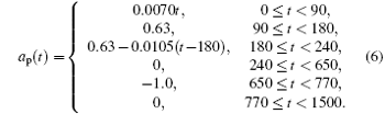
Suppose that the initial state of vehicle following system is described as follows: sf0 = 0 m, dactual0 = 6500 m, vp0 = 20 m/s, vf0 = 45 m/s, ape = − 1.0 m/s2, δ = 5%, and η = 0.5 m/s. As the dotted lines shown in Figs. 7 and 8, the preceding vehicle moves forward at the corresponding acceleration and velocity in the following equation:
According to the above calculation method of the control laws for vehicle following system, the following vehicle can adjust its own behavior to adapt the dynamic behavioral change of the preceding vehicle, as seen in Figs. 7 and 8.
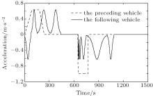
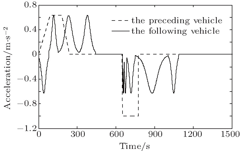 | Fig. 7. Acceleration– time curves of the preceding and following vehicles. |
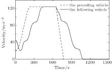
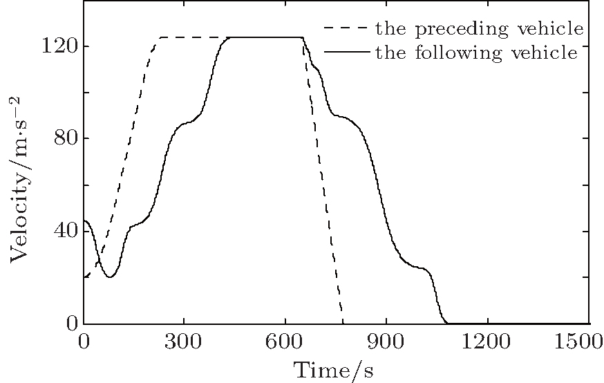 | Fig. 8. Velocity– time curves of the preceding and following vehicles. |
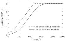
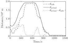
There may be collision risk if the following vehicle moves faster than the preceding vehicle all the time. In order to follow the “ safety first” principle, the following vehicle slows down from 45 m/s to about 20 m/s at the beginning of its behavioral adjustment (see Figs. 7 and 8). And then, the following vehicle begins to speed up to improve the efficiency when its velocity is less than or equal to that of the preceding vehicle (see Figs. 7 and 8). The preceding vehicle should not always change its behavior unless it must adjust its own behavior. In fact, avoiding the frequent behavioral adjustment needs to be taken into consideration in the design and construction stages of the highway or motorway. When the preceding vehicle travels at a constant velocity, the following vehicle will adjust its own behavior to establish a new safe and efficient steady-following state at 443 s with a velocity of 120 m/s and Δ d = 532.0 m, as shown in Figs. 7– 11. However, when the safe and efficient steady-following state is broken from 650 s by the preceding vehicle’ s slowing down to stop, a new behavioral adjustment is adopted by the following vehicle to respond to the stopping of the preceding vehicle until a special safe and efficient steady-following state, i.e., the state of rest, is re-established with Δ d = 218.0 m as shown in Figs. 7– 10. In Refs. [61] and [62], the acceleration and jerk were used to evaluate the smoothness (comfort) of vehicle movement. Castellanos and Fruett[63] constructed an embedded system in which the acceleration and jerk magnitudes were used to evaluate the passenger comfort in public transportation. Generally, vehicle movement is judged to be smooth (comfortable) under the absolute value of acceleration not greater than 0.63 m/s2[59, 60] and absolute value of jerk not greater than 2.0 m/s3.[61, 62] Figures 8 and 11 display the good smoothness (comfort) of the following vehicle’ s behavioral adjustment. Figure 10 verifies the safety and efficiency of vehicle following system with the control laws given by the proposed mathematical models constructed by the hyperbolic functions. It is worth pointing out that the synchronous control of af, Δ v, and Δ d can be well realized by the integrated application of the proposed mathematical models, as shown in Figs. 7– 10.
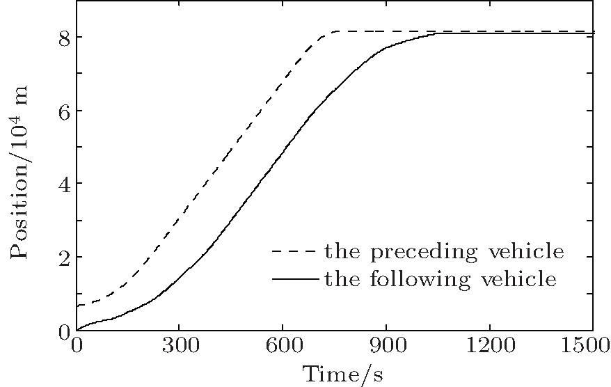 | Fig. 9. Position– time curves of the preceding and following vehicles. |
 | Fig. 10. Distance– time curves of the preceding and following vehicles. |
Clearly, attention was not paid to the synchronous control of af, Δ v, Δ d and in the OV model, [6, 7] the FVD model, [10] the FVAD model, [11] or the FVDA model.[52] As mentioned above, the purpose of vehicle following control is just to establish, maintain, and re-establish the previous or new safe and efficient steady-following state, not to change their own behaviors endlessly. To establish, maintain, and re-establish the safe and efficient steady-following state, only the synchronous control of af, Δ v, and Δ d can help vehicle following system achieve this purpose.
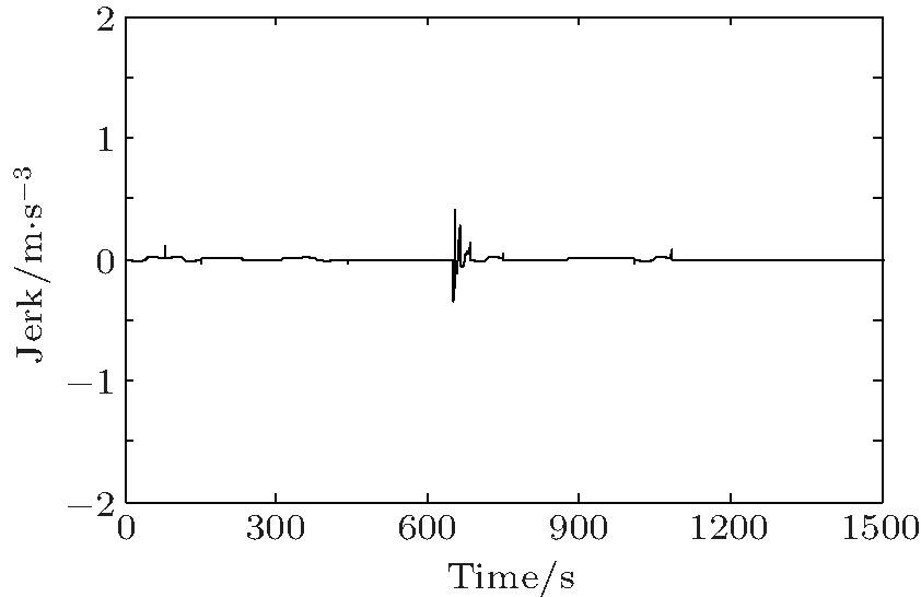 | Fig. 11. Jerk– time curve of the following vehicle. |
In addition, from some literature, such as Refs. [24], [51]– [54], [56], and [57], we can see that the hyperbolic tangent function was used to study the vehicle following system. In their established mathematical models the optimal velocity of each vehicle changes with spatial headway or the actual following distance. Newell[24] admitted that, “ Indeed, the theory has a number of serious deficiencies. It contains the implication that drivers follow one another under nonstationary conditions by adhering to the same velocity-headway relation they would choose under steady conditions.” By contrast, neither the spatial headway nor the actual following distance appears in our mathematical models built using the hyperbolic functions. As for which one of our mathematical models is to be used by the following vehicle to adjust its own behavior depends on our judgment of the vehicle following situation (see Fig. 6). On the other hand, the setting of some parameters, such as the uniform initial headway and the constant safety distance, may not reflect the complex and time-varying situation of vehicle following operation because these parameters always change with vehicle following situation. Comparatively speaking, our models have stronger adaptive ability for vehicle following control.
Based on our understanding of vehicular behavior adjustment and vehicle distance control, in this paper the hyperbolic functions are used to describe the behavioral adjustment process of the following vehicle. And then the control laws of the following vehicle adjusting its own behavior are calculated according to the quality evaluation of vehicle following behavior in safety, efficiency, and smoothness (comfort). From the above simulation and analysis, we can see that the following vehicle can follow the “ safety first” principle and adjust its own behavior in safety, efficiency, and smoothness (comfort) until a new safe and efficient steady-following state is re-established. However, the time delay is not considered by the control laws in the behavioral adjustment of the following vehicle. In our future study, more attention will be paid to this problem and we will try to give a strict proof to the safety and efficiency of the control laws calculated by the hyperbolic functions.
| 1 |
|
| 2 |
|
| 3 |
|
| 4 |
|
| 5 |
|
| 6 |
|
| 7 |
|
| 8 |
|
| 9 |
|
| 10 |
|
| 11 |
|
| 12 |
|
| 13 |
|
| 14 |
|
| 15 |
|
| 16 |
|
| 17 |
|
| 18 |
|
| 19 |
|
| 20 |
|
| 21 |
|
| 22 |
|
| 23 |
|
| 24 |
|
| 25 |
|
| 26 |
|
| 27 |
|
| 28 |
|
| 29 |
|
| 30 |
|
| 31 |
|
| 32 |
|
| 33 |
|
| 34 |
|
| 35 |
|
| 36 |
|
| 37 |
|
| 38 |
|
| 39 |
|
| 40 |
|
| 41 |
|
| 42 |
|
| 43 |
|
| 44 |
|
| 45 |
|
| 46 |
|
| 47 |
|
| 48 |
|
| 49 |
|
| 50 |
|
| 51 |
|
| 52 |
|
| 53 |
|
| 54 |
|
| 55 |
|
| 56 |
|
| 57 |
|
| 58 |
|
| 59 |
|
| 60 |
|
| 61 |
|
| 62 |
|
| 63 |
|