
Estimation of random errors for lidar based on noise scale factor
[Wang Huan-Xuea), b) , Liu Jian-Guo†b)  , Zhang Tian-Shu
b) ]
, Zhang Tian-Shu|
|


†Corresponding author. E-mail: jgliu@aiofm.ac.cn
*Project supported by the Strategic Priority Research Program of the Chinese Academy of Sciences (Grant No. XDB05040300) and the National Natural Science Foundation of China (Grant No. 41205119).
Estimation of random errors, which are due to shot noise of photomultiplier tube (PMT) or avalanche photodiode (APD) detectors, is very necessary in lidar observation. Due to the Poisson distribution of incident electrons, there still exists a proportional relationship between standard deviation and square root of its mean value. Based on this relationship, noise scale factor (NSF) is introduced into the estimation, which only needs a single data sample. This method overcomes the distractions of atmospheric fluctuations during calculation of random errors. The results show that this method is feasible and reliable.
Lidar has been used for atmospheric remote detection by Fiocco and Smullin[1] since laser was invented. In recent years, the development of laser technology well enhanced the laser power, and the progress of photoelectric technology improves the detection sensitivity of lidar. Due to its high spatiotemporal resolution, lidar has been used as a powerful tool for the global observation of atmospheric compositions, such as wind, clouds, water vapor mixing ratio, aerosols, etc.[2– 6] There exist two major types of uncertainties, [7] i.e., random errors and systematic errors, in lidar observation. The random errors, which are inevitable in lidar measurement, result from three sources: (i) quantum noise, (ii) thermal noise, and (iii) excess noise which is caused by multiplication process. The random errors can be minimized by multiple measurements. Compared with random errors, the systematic errors can produce a certain offset that cannot be reduced by average measurements. In this paper, we focus our discussion on random errors and methods for their estimation.
Multiple-measurement is widely used as a traditional method to estimate random errors for lidar measurements. The average signal value and random errors can be obtained by averaging measurements at the same height. All data collected every time are required to be stored in the traditional method. So the data storage of this method is large. The traditional method is based on a principle that the signal is not changed during the measurement. However, the natural variability of the atmosphere can cause significant fluctuation of signal, which can be often detected as random errors by mistake. These random errors may bring about a great influence on the composition measurement while the atmospheric parameters changes rapidly (e.g., windy and cloudy).
In what follows, we introduce noise scale factor (NSF) into the calculation of random errors, in which only a group of discrete-distance signals is used. This method overcomes the distractions of atmospheric fluctuations during the calculation of random errors. The results show that using NSF to estimate random errors is feasible and reliable.
In lidar observations, the backscatter signal is very small, so a set of dynodes or secondary-emitting electrodes is employed, which can give a large current or voltage gain. However, because of the variation of secondary-emitting gain, excess noise is produced in the multiplication process in a PMT or APD.[8] Noise factor F can be used to parameterize the excess noise.
Also, F can be derived from the moment-generation function, F at the j-th dynode stage can be described from[8]
And when j → ∞ , equation (1) can be expressed as

Meanwhile, the magnification coefficient of photomultiplier can be given as

where m is the multiplication factor and n is the number of dynode stage of a PMT. From Eqs. (1) and (2), we can find that for higher m, F is smaller, G is larger. Consequently, a high value of multiplication factor can produce large gain and small excess noise. For PMTs, F varies from 1 to 2 with a maximum value of 1.5.[9]
The mean and standard deviations of total output electrons at the j-th dynode stage are described by[8]


Here, Qin is the mean of total incident photoelectrons and expressed as

where Qs is the lidar backscatter signal, Qb is the solar radiation, and Qd is the dark current.
In lidar detection, PMT or APD converts a light signal into an electrical signal in two ways: AD conversion and photon counting. In this paper, we focus our discussion on PMT.
The noise of lidar signal usually includes sky background signal and dark current of detector. Even if the number of photons emitted from the laser is representative of constant intensity, the number of photons arriving at the detector is uncertain due to the quantum nature of the laser light. The theory and experiments show that if the photons arriving rates are independent of time, the photon number arriving in any given time yields a random Poissonian distribution.[10, 11] Based on the Poissonian distribution, the variance of the number of photons emitted from the laser is equal to its mean, so that

where np represents the number of photons emitted from the laser, and σ np represents the variance of np.
In actual practice, when a PMT operates in an AD conversion mode, even if the incident photons follow Poissonian distribution, due to the excess noise produced by photoelectron multiplication in PMT, the output electrons of the anode do not follow the distribution.[8, 11, 12] In this case, the variance of output electron 


where σ ne is the variance of ne.
When the detector operates in a photon counting mode, the output quantity is photoelectron and if the detector works in an AD conversion mode, the output quantity is voltage or current. In this case, the relationship between photoelectron

where τ is the detection time.
As shown by the above discussion, the NSF is introduced to estimate the standard deviation, σ x, of a measurement x, where,

For a photon counting mode, NSF = 1. For the AD conversion mode, if the output quantity is photoelectron, the NSF is given by

If the output quantity is current or voltage, the NSF is given by

Here, e is the electron charge, B is the spectral bandwidth of detector, and B ≈ 1/2τ , G′ represents the gain factor that converts the anode current of the detector into digital signal (digitizer counts). By Eq. (9b), the NSF is related to the output quantity and hardware parameters of detector.
In practice, there are two main noise sources existing in the lidar measurements . One is the solar radiation, another is the detector dark current. Thus, each digitized sample, Q, can be written as Q = Qs + Qb + Qd, the variance of Q can be written as

where Δ Qs (the variance of Qs), Δ Qb (the variance of Qb), and Δ Qd (the variance of Qd) can be obtained by NSF respectively,

where 


Because

where Nb represents the number of lidar signal profiles from which
Based on Eq. (8), the NSF can be derived by using
Equation (14) represents the NSF measurement in daytime (the solar radiation is dominant). When the measurement is conducted under nighttime condition, the dark current cannot be ignored, equation (14) can be re-written as

In these equations above, Δ Qb and Δ Qd represent the standard deviation of the background signal and dark current, respectively.
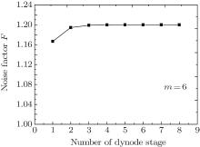
In our lidar observation, the parameters in Eq. (1b) are all known, noise factor F can be calculated straightforwardly. Figure 1 shows F of each dynode stage as obtained from Eq. (1b). From Fig. 1, it can be seen that as j is larger than 3, Fj is roughly equal to a maximum value of 6/5, and after the third dynode stage, the F value is approximately constant.
 | Fig. 1. Noise factors at different dynode stages, derived from Eq. (1b). |
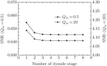
The two cases, i.e., Qin = 0.5 and Qin = 20, are considered. The output SNRs, which are equal to Qout, j/σ out, j, are presented in Fig.2. As can be seen from Fig. 2, when j is larger than 3, the SNRs are 0.645 and 4.082, respectively, for different values of Qin. This further supports the above conclusion. Meanwhile, the output SNRs are smaller than the input SNRs, 0.707 and 4.472, and the output SNRs are equal to (Qin)1/2, suggesting that the multiplication process in a PMT or APD can produce the excess noise.
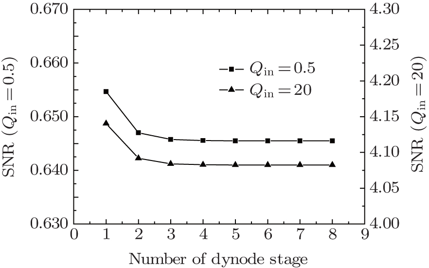 | Fig. 2. Output SNRs at different dynode stages. |
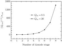
Figure 3 shows the square root and standard deviations of output electrons at different stages for different values of Qin. From Fig. 3, it can be seen that there is a proportional, one-to-one relationship existing between the square root and standard deviation of its means. Figure 4 gives this one-to-one relationship.
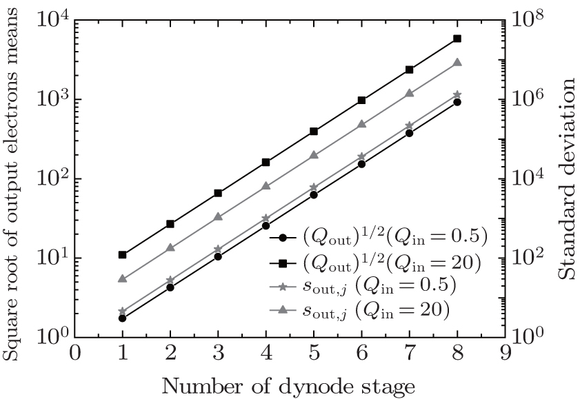 | Fig. 3. Square root and standard deviations of output electrons at different dynode stages, obtained from Eqs. (3a) and (3b). |
 | Fig. 4. (Qout)1/2/σ out at different dynode stages for different values of Qin. |
As can be seen from Fig. 4, the value of (Qout)1/2/σ out is irrespective of Qin, and it is related to F and G only.
Because of the excess noise, which is produced by the multiplication process in PMTs or APDs, even if the incident photons follow Poisson statistics, the multiplied carriers do not follow Poisson distribution. In spite of this, a proportional, one-to-one relationship between standard deviation and square root of its means still exists in PMTs and APDs.[7] Based on this relation, NSF is introduced into the estimation of random errors.
As can be seen from Eqs. (9a) and (9b), in principle, the NSF value is determined by parameters of detectors. However, in real application, we usually compute the mean and standard deviation from measurement data, and then obtain the NSF value derived from Eqs. (14) and (15).
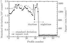
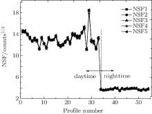
The standard deviation of background can be calculated by computing the standard deviation over a set of samples in each signal profile. We must select the samples from a region where the lidar backscatter signal is nearly ignored. Figure 5 shows the square root and standard deviation of background signal, which are derived from the high altitude region for lidar measurement at San Men Xia on January. 1, 2014. It is shown that when the measurement is performed in the daytime, the dominant background noise signal is solar radiation. The NSF is shown in Fig. 6, which is derived by using Eq. (14).
 | Fig. 5. Standard deviations and square roots of lidar signals. |
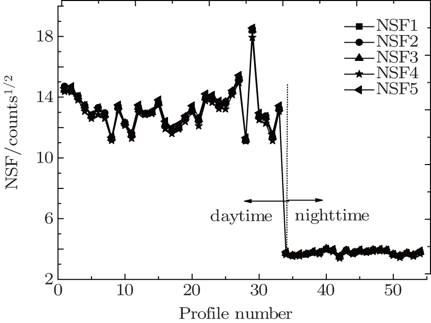 | Fig. 6. NSF calculations by using Lidar signal. |
We select the detection data of five days, which are selected by the same lidar system, to calculate NSF and the weather conditions of the five days have little difference. The results are shown in Fig. 6. From Fig. 6 it can be seen that the NSF changes gently under daytime measurement condition. However, there is a sudden change in NSF at profile number 25. The sudden changes for the profile numbers from 25 to 30 are caused by saturation of the background monitor digitizer, which can be seen from Fig. 6. The NSF of nighttime is smaller than that of daytime, that is because, in nighttime, the solar radiation is very weak, and the dark current is the dominant background noise signal source.
We note that the NSF is dependent only on measurement signal domain.[7] So, if the value of the domain is a constant, the value of NSF, which is obtained from the domain, is a constant. And it is more convenient to use the NSF for estimating the random errors of the domain. However, for attenuated backscatter coefficients or extinction coefficients domain, NSF is a function of detection height, and it is not a constant.
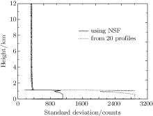
Figure 7 shows the standard deviations derived from lidar measurements using photon counting detection in two ways: one is computed for each altitude bin by using 20 consecutive profiles, and the other is computed by using the NSF .
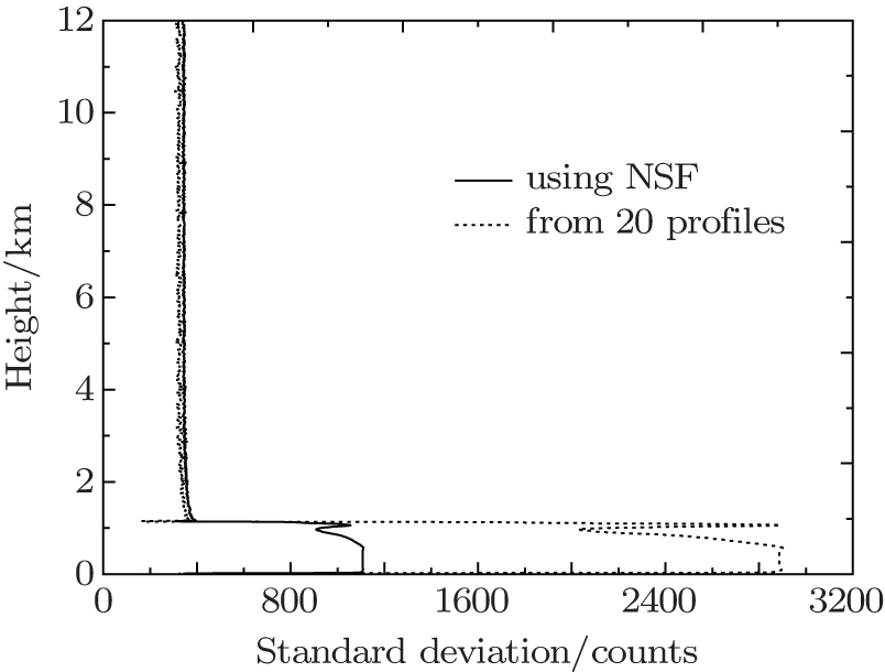 | Fig. 7. Profiles of standard deviation lidar signal, obtained by using NSF and conventional method. |
As seen from Fig. 7, in the aerosol-free region (i.e., above 1.5 km), the standard deviations computed from 20 profiles are consistent with those which are derived from NSF, which is because atmospheric molecular scattering dominates the upper atmosphere, and atmospheric molecules change little over time. At an altitude below 1.5 km, the uncertainties decrease with increase in altitude. And apparently, the results from these two methods are in disagreement with each other, the results of conventional method is larger than those calculated using NSF. It is because the aerosol has a great fluctuation below 1.5 km. In the conventional method, this fluctuation is mistaken for the random error of lidar signal, so this method significantly overestimates the random error. This result proves the reliability of NSF in random error calculation.
Based on our results above, when using the conventional method, the natural fluctuation of atmosphere can produce significant overestimation of random error of lidar signal. This effect is much more severe in those area where atmosphere changes dramatically. Compared with the results from the traditional method, with NSF, the random error can be computed from a single sample, and the result will not be influenced by atmosphere change. So, in the estimating of random errors, the use of NSF has an obvious advantage over traditional method.
For lidar measurement, random error and systematic error must be considered. In this paper we focus our discussion on the random error. In general, the random error is estimated by computing the standard deviation of a series of consecutive signal samples. But its application requires a large number of lidar data samples, and this method is obviously influenced by the natural variability of the atmosphere. So in boundary layer, where the atmospheric composition changes rapidly, this method will produce large errors.
By using NSF to calculate random error of lidar signal, only one data sample is needed, so the result is not influenced by the atmospheric fluctuations and makes up for a shortage of the conventional method. The background signal and dark current, which determine the value of NSF, can be measured directly. The results show that when in the daytime condition, NSF is not influenced by dark current. That is because compared with background signal, dark current is so small that its effect can be ignored. But in the nighttime, the dark current has a significant influence on NSF. Meanwhile, NSF can be calculated accurately, which can improve the accuracy of the estimation of random errors due to lidar. The comparison between the results from these two methods shows that in the estimation of the random errors of lidar signal, NSF is feasible and reliable.
| 1 |
|
| 2 |
|
| 3 |
|
| 4 |
|
| 5 |
|
| 6 |
|
| 7 |
|
| 8 |
|
| 9 |
|
| 10 |
|
| 11 |
|
| 12 |
|