Qiu Yang, Li Hua, Zhang Shu-Lin, Wang Yong-Liang, Kong Xiang-Yan†, Zhang Chao-Xiang, Zhang Yong-Sheng, Xu Xiao-Feng, Yang Kang, Xie Xiao-Ming. Low- Tc direct current superconducting quantum interference device magnetometer-based 36-channel magnetocardiography system in a magnetically shielded room . Chinese Physics B, 24(7): 078501
Permissions
Low- Tc direct current superconducting quantum interference device magnetometer-based 36-channel magnetocardiography system in a magnetically shielded room
Qiu Yanga),b),c), Li Huaa),b),c), Zhang Shu-Lina),b), Wang Yong-Lianga),b), Kong Xiang-Yan†a),b), Zhang Chao-Xianga),b), Zhang Yong-Shenga),b), Xu Xiao-Fenga),b), Yang Kanga),b),c), Xie Xiao-Minga),b)
State Key Laboratory of Functional Materials for Informatics, Shanghai Institute of Microsystem and Information Technology, Chinese Academy of Sciences, Shanghai 200050, China
Joint Research Laboratory on Superconductivity and Bioelectronics, Collaboration between Chinese Academy of Sciences–Shanghai, Shanghai 200050, China and FZJ, D-52425 Julich, Germany
University of Chinese Academy of Sciences, Beijing 100049, China
*Project supported by “One Hundred Persons Project” of the Chinese Academy of Sciences and the Strategic Priority Research Program (B) of the Chinese Academy of Sciences (Grant No. XDB04020200).
Abstract
We constructed a 36-channel magnetocardiography (MCG) system based on low- Tc direct current (DC) superconducting quantum interference device (SQUID) magnetometers operated inside a magnetically shielded room (MSR). Weakly damped SQUID magnetometers with large Steward–McCumber parameter βc ( βc ≈ 5), which could directly connect to the operational amplifier without any additional feedback circuit, were used to simplify the readout electronics. With a flux-to-voltage transfer coefficient ∂ V/ ∂ Φ larger than 420 μV/ Φ0, the SQUID magnetometers had a white noise level of about 5.5 fT·Hz−1/2 when operated in MSR. 36 sensing magnetometers and 15 reference magnetometers were employed to realize software gradiometer configurations. The coverage area of the 36 sensing magnetometers is 210×210 mm2. MCG measurements with a high signal-to-noise ratio of 40 dB were done successfully using the developed system.
Magnetocardiography (MCG) is a non-invasive technique which employs extremely sensitive devices such as superconducting quantum interference devices (SQUIDs) to record and analyze the magnetic field signals generated from the ionic current activity of heart muscle. It has been demonstrated to be very helpful for the diagnoses of myocardial ischemia and localization of arrhythmic current paths.[1] To speed up the measurement, several multichannel MCG systems were developed, and the sensor coverage area is large enough to simultaneously get the major cardiac magnetic field which was changed with space.[2– 4]
As a magnetic flux detector, SQUID is of high sensitivity for the measurement of weak biomagnetic fields such as magnetocardiography and magnetoencephalography (MEG).[5] The SQUID readout electronics which amplify the small SQUID output signals will introduce additional noise from the room-temperature preamplifier. Traditionally, the flux modulation technique is introduced to suppress the preamplifier noise.[6] However, for a multi-channel MCG system, the flux modulation technique will substantially increase the system complexity. For that reason, several direct readout schemes, such as additional positive feedback (APF), [7] noise cancellation (NC), [8] as well as SQUID bootstrap circuit (SBC), [9] which suppress the preamplifier noise without flux modulation, have been introduced to simplify the SQUID readout electronics. Recently, it has been shown that a weakly damped niobium-SQUID with a large Steward– McCumber parameter β c (> 1) could directly connect to an operational amplifier without any additional feedback circuit and further simplify the readout electronics.[10] The large β c can provide a large flux-to-voltage transfer coefficient ∂ V/∂ Φ , thus reducing the preamplifier noise contribution, δ Φ preamp. This kind of SQUID is well suited for SQUID systems with a large number of channels.
In this paper, we report a low-noise 36-channel MCG system based on weakly damped low-Tc direct current (DC) SQUID magnetometers in a magnetically shielded room (MSR). In order to avoid the complicated fabrication process of coil gradiometers, we use the software gradiometer as the magnetic field detector. In addition, we compared the MCG signal characteristics measured with different software gradiometers under the same measurement condition.
2. Experiment setup
The schematic diagram of the 36-channel MCG system in a magnetically shielded room is depicted in Fig. 1. The insert consists of 36 signal sensors, 12 reference sensors, and a 3-axis vector reference module spread on three separate layers, respectively. A low noise non-magnetic liquid helium fiberglass cryostat with 28 L volume will supply the low temperature environment. We hung it on a gantry and adjusted its vertical position from above as close as possible to the patient’ s chest. The patient bed is also made of non-magnetic materials and can be moved in two directions for the fine adjustment of the measurement location. Readout electronics which connect to the SQUIDs were mounted on top of the cryostat. A SQUID readout controller (SRC) which sets the SQUID bias current, voltage offset, reset switch, and FLL switch, was installed outside of a MSR connected with a data acquisition system (DAS) and personal computer. The MSR has shielding factors of 46 dB at 0.1 Hz and 61 dB at 1 Hz.
Fig. 1. Schematic configuration of the 36-channel MCG system.
2.1. SQUID magnetometer
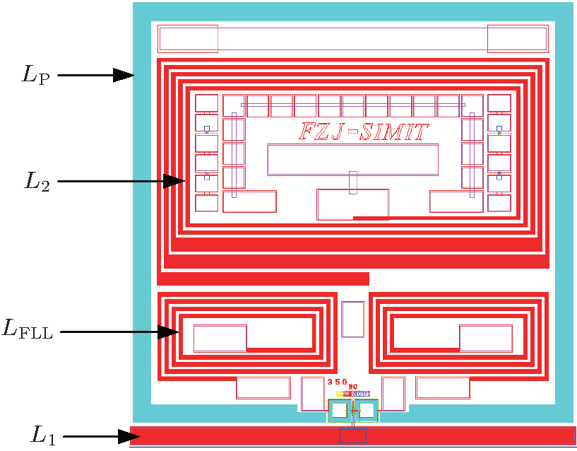
In our experiments, dual-washer SQUID magnetometers with a designed loop inductance Ls = 350 pH were employed. The complete layout of our SQUID on a chip of size 10× 10 mm2 is shown in Fig. 2. Here, the junction shunted resistance RJ = 30 Ω is designed to provide a large β c ≈ 5, thus increasing the ∂ V/∂ Φ and suppressing the preamplifier noise. A flux feedback coil LFLL with 4 turns for the flux locked loop (FLL) operation, a heating resistor Rh for removing trapped flux and two opposite input coils Lin, which connected in series with the on-chip pickup loop Lp, integrated on the SQUID-washer are also included in the design. Two planar coils, L1 and L2, which can be used to implement suitable current and voltage feedbacks of SBC, were also integrated in the design as an option. The flux-to-field coefficient ∂ B/∂ Φ of the magnetometers is measured to be about 0.55 nT/Φ 0. Table 1 shows the designed parameters of the SQUID chip.
Fig. 2. Layout of the SQUID chip with a size of 10× 10 mm2.
Table 1.
Table 1.
Table 1. Design parameters of the SQUID chip.
Parameter
Value
Unit
Chip size
10× 10
cm2
One junction size
3× 3
μ m2
Junction resistance RJ
30
Ω
Junction critical current I0
4
μ A
SQUID loop inductance Ls
350
pH
Turns of LFLL
4
/
Turns of Lin
5× 2
/
Heating resistance Rh
131
Ω
Table 1. Design parameters of the SQUID chip.
2.2. Readout electronics
The SQUID is connected to the readout electronics with FLL at room temperature via a cryogenic cable (see Fig. 3(a)). A commercial operational amplifier (OP) AD797 with a voltage noise Vn of 1 nV· Hz− 1/2 is chosen as the preamplifier of the FLL electronics. The SQUID is directly connected to the inverting input of the OP while the bias voltage Vb is applied at the non-inverting input. The OP acts as a current-to-voltage converter in our experiments with voltage-biased SQUIDs.
Fig. 3. (a) Schematic diagram of voltage-biased SQUID connecting to a current-to-voltage convertor. Here, Vb is the bias voltage. (b) The photo of a 4-channel FLL electronics. (c) The photo of 64-channel SQUID readout controller.
The PCB board of each FLL electronics has a size of 38× 22 mm2, and 4 FLL PCBs were assembled in an aluminum box with a size of 123 mm× 110 mm× 27 mm (see Fig. 3(b)). In total, 13 aluminum boxes were mounted on top of the Dewar for the 36-channel MCG system. FLL electronics were control by the SQUID readout controller, which set the SQUID bias current, voltage offset of the integrator, reset switch, FLL switch, and filter switches. The output of FLL electronics was collected with 24-bit A/D cards (NI PCI-4472) with a sampling rate of 1 kHz. The data were stored in a computer for further processing. The SQUID readout controller, data acquisition system and computer were installed outside of the MSR.
2.3. Insert configuration
The arrangement of the 36 sensing magnetometers and 15 reference magnetometers is illustrated in Fig. 4. The magnetometers are located in three layers. The lowest is called a sensor layer. The distance between the nearest adjacent sensing magnetometers in sensor layers is about 38 mm. The coverage area of the sensing magnetometers is 210 × 210 mm2. The middle is called the reference layer and the uppermost is a 3-axis reference layer. The vertical distance between neighboring layers is 70 mm. Among the 51 channels, a total of 49 magnetometers are orientated to detect vertical field components, and 2 magnetometers to detect horizontal components. Using reference magnetometers, one can construct a software gradiometer to eliminate environmental noises.
Fig. 4. Schematic arrangement of sensing magnetometers and reference magnetometers.
3. Results and discussion
3.1. Statistical characterization of SQUIDs
We prepared and measured 52 SQUID magnetometers of the layout discussed above, having a nominal RJ = 30 Ω . All 52 SQUIDs can be stably operated in the voltage bias mode as the direct readout scheme of Fig. 2, no obvious instability was observed. Figure 5(a) illustrates the spread of current swing Iswing. The Iswing mean value of 4 μ A corresponds to ∂ i/∂ Φ of about 12 μ A/Φ 0 at the working point, while the Rd mean value is about 35 Ω . Due to the large β c (β c ≈ 5), the SQUIDs exhibit a large ∂ V/∂ Φ = (∂ i/∂ Φ )Rd = (12 μ A/Φ 0) (35 Ω ) ≈ 420 μ V/Φ 0. The equivalent flux noise of the preamplifier, δ Φ preamp = Vn/(∂ V/∂ Φ ), is estimated to be 2.4 μ Φ 0· Hz− 1/2. In this case, the noise contribution of the preamplifier was effectively suppressed. We measured the SQUIDs noise while the SQUID magnetometers were shielded by placing them in a niobium tube, and we also measured the single-channel noise while the SQUID magnetometers were not shielded by placing them in a non-magnetic liquid helium fiberglass cryostat in the MSR. Figure 5(b) shows the SQUIDs noise and the single-channel noise of the SQUID magnetometers. Statistically, 90% of the SQUIDs noise was below 10 μ Φ 0· Hz− 1/2. The field sensitivity δ B, a product of the flux-to-field transfer coefficient (∂ B/∂ Φ ) and the flux sensitivity δ Φ i.e., δ B = (∂ B/∂ Φ )δ Φ reaches about 5.5 fT· Hz− 1/2. Figure 5(c) shows a typical noise spectrum of all the SQUID magnetometers measured with a superconducting shielding and in non-magnetic cryostat in MSR respectively. The results showed that it meets the need for MCG signal measurement.
Fig. 5. Statistical characterizations of the voltage-biased SQUID magnetometers: (a) Iswing; (b) SQUID noise, (c) the noise measurements of a typical noise spectrum measurement of the SQUID magnetometers, whose ∂ B/∂ Φ is measured to be 0.55 nT/Φ 0.
3.2. System calibration
When multi-channel SQUID magnetometers are used for biomagnetic applications, the correct measurement of the proportionality between the output voltage of the magnetometer and the magnetic field is of extreme importance. We designed and fabricated a two-square-loop uniaxial Helmholtz coil system for calibration. Each coil is 1750 mm× 1750 mm in size. Coil frames are made of wood and assembled by nylon screws.
To minimize noise effects we calibrated our system inside the MSR. We used an ac current of 13 Hz to generate uniform field source Δ B and the SQUID magnetometers responded to a voltage change Δ V. Using Biot– Savart’ s law, we obtained an analytical expression of the magnetic field in all space. The proportionality between the output voltage of the magnetometer and magnetic field of each channel is calculated to be about 1.6 pT/mV.
3.3. MCG measurements
Based on the above system, the MCG signal detection of an adult is demonstrated inside the MSR. The MCG signals were sampled with the data acquisition system and stored in a personal computer. In order to remove the disturbance from the ambient, such as the power line interference, a low-pass FIR filter with a cut-off frequency of 150 Hz and a notch filter of 50 Hz were employed for the data processing. The typical measurement time was 30 s. The liquid helium cryostat has an internal diameter of 300 mm, and an internal length of 900 mm. The volume of the Dewar is 28 L, and the boil-off rate of liquid helium is about 4.7 L/d in everyday operation of the MCG system. The cryostat can be moved vertically to adjust its height. The bed for a subject to lie on is made of nonmagnetic materials and can be moved in two directions for the fine adjustment of the measurement location.
Software gradiometers can be combined using one sensing magnetometer with different reference magnetometers. The output of the software gradiometer will become BG = S − K1R1 − K2R2 − K3R3, in which S is the output of the sensing magnetometer, R1, R2, and R3 are the outputs of reference magnetometers and K1, K2, and K3 are coefficients. The constant coefficients can be obtained by a least square rule similar to the method used in Ref. [11]. Figure 6(a) shows the MCG signals measured using different software gradiometers: Figure 6(a) shows the MCG signals measured using one sensing magnetometer S02 with different reference magnetometers: (I) reference magnetometer R01, (II) reference magnetometer R15, and (III) 3-axis reference. The measured MCG signals increase from 65 pT (I) to 95 pT (II) and then to 105 pT (III). This result means that software gradiometers with longer baselines give better SNR due to large signal amplitudes. This is because the gradiometer, whose baseline is too short, cancels out not only the noise but also the signal. A well working R15 needs a higher liquid helium level, so we finally chose 4 SQUIDs which were located at the outer place of the middle level, just like R01, as reference magnetometers, and each reference magnetometer compensates a 3× 3 sensing magnetometers array (see Fig. 4).
Fig. 6. (a) A 28-year old adult’ s MCG signals measured using one sensing magnetometer S02 with different reference magnetometers. (b) Real-time MCG signals measured using the 36-channel system. (c) The MCG magnetic field map.
Figure 6(b) shows real-time MCG traces of a 36-channel MCG system. The analysis software provides magnetic field mapping (see Fig. 6(c)). From the above mapping, useful clinical parameters such as the angle between negative and positive poles, the maximum change map of the map angle, and the maximum distance change between the centers of negative and positive poles, can be obtained.
4. Conclusion
Based on a weakly damped niobium-SQUID, a 36-channel MCG system was set up in MSR. Readout electronics without any additional feedback circuit were used to read out the MCG signals. Operated inside a MSR, the average white noise level of the system was about 5 fT· Hz− 1/2. The recorded MCG signal displays a high SNR of 40 dB. Using the above MCG data array, magnetic field maps (MFM) and some useful clinical parameters could be obtained.
... [1] To speed up the measurement, several multichannel MCG systems were developed, and the sensor coverage area is large enough to simultaneously get the major cardiac magnetic field which was changed with space ...
1
1995
0.0
0.0
... [2#cod#x2013 ...
1
2009
0.0
0.0
1
2013
0.0
0.0
... 4] ...
1
2004
0.0
0.0
... [5] The SQUID readout electronics which amplify the small SQUID output signals will introduce additional noise from the room-temperature preamplifier ...
1
1967
0.0
0.0
... [6] However, for a multi-channel MCG system, the flux modulation technique will substantially increase the system complexity ...
1
1990
0.0
0.0
... For that reason, several direct readout schemes, such as additional positive feedback (APF),[7] noise cancellation (NC),[8] as well as SQUID bootstrap circuit (SBC),[9] which suppress the preamplifier noise without flux modulation, have been introduced to simplify the SQUID readout electronics ...
1
1995
0.0
0.0
... For that reason, several direct readout schemes, such as additional positive feedback (APF),[7] noise cancellation (NC),[8] as well as SQUID bootstrap circuit (SBC),[9] which suppress the preamplifier noise without flux modulation, have been introduced to simplify the SQUID readout electronics ...
1
2010
0.0
0.0
... For that reason, several direct readout schemes, such as additional positive feedback (APF),[7] noise cancellation (NC),[8] as well as SQUID bootstrap circuit (SBC),[9] which suppress the preamplifier noise without flux modulation, have been introduced to simplify the SQUID readout electronics ...
1
2012
0.0
0.0
... [10] The large #cod#x03B2 ...
1
2012
0.0
0.0
... [11] ...
Low- Tc direct current superconducting quantum interference device magnetometer-based 36-channel magnetocardiography system in a magnetically shielded room
[Qiu Yanga),b),c), Li Huaa),b),c), Zhang Shu-Lina),b), Wang Yong-Lianga),b), Kong Xiang-Yan†a),b), Zhang Chao-Xianga),b), Zhang Yong-Shenga),b), Xu Xiao-Fenga),b), Yang Kanga),b),c), Xie Xiao-Minga),b)]


 , Zhang Chao-Xiang