


Nonlinear tunneling through a strong rectangular barrier
[Zhang Xiu-Rong, Li Wei-Dong† ]
]
]
|
|


†Corresponding author. E-mail: wdli@sxu.edu.cn
*Project supported by the National Natural Science Foundation of China (Grant Nos. 11074155 and 11374197), the Program for Changjiang Scholars and Innovative Research Team in University (PCSIRT), China (Grant No. IRT13076), and the National High Technology Research and Development Program of China (Grant No. 2011AA010801).
Nonlinear tunneling is investigated by analytically solving the one-dimensional Gross–Pitaevskii equation (GPE) with a strong rectangular potential barrier. With the help of analytical solutions of the GPE, which can be reduced to the solution of the linear case, we find that only the supersonic solution in the downstream has a linear counterpart. A critical nonlinearity is explored as an up limit, above which no nonlinear tunneling solution exists. Furthermore, the density solution of the critical nonlinearity as a function of the position has a step-like structure.
Since the first experimental realization of Bose– Einstein condensates (BECs) in 1995, [1– 3] nonlinear tunneling, as a pedagogic quantum problem, has been explored both experimentally and theoretically. From the experimental perspective, it could be investigated by moving a laser beam (as a potential) through elongated BECs or exciting the collective dipole oscillation of BECs in an optical harmonic trap with different additional defects.[4– 7]
However it is difficult to find analytical results for the nonlinear case in which the superposition principle is broken down. For restricted systems, such as BECs in a harmonic trap, in a double or triple well, or in an optical lattice, some numerical or theoretical methods have been employed to solve the Gross– Pitaevskii equation (GPE), for example, two- or three-mode approximation, the symplectic method, and the particle swarm optimization (PSO) algorithm.[8– 14] For non-restricted systems, a few methods have been proposed to deal with the nonlinear tunneling problem from various aspects, for example, involving the nonlinear effect only within the barrier, [15] or gradually increasing nonlinear interaction as BECs approaching an atomic quantum dot in a waveguide.[16] The dispersive wave shocks, formed in the upstream when BECs collide with a potential, were suggested to be studied by hydromechanics methods (Riemann invariants).[17, 18] With the help of numerical solutions of the GPE, different stationary density solutions of BECs through a waveguide with a disturbing obstacle have been reported.[19, 20] It has been proved that the behaviors of the density solutions dramatically depend on the velocity of the BECs and the size and strength of the obstacle. For a supersonic BEC and a strong potential barrier, a step-like density is formed when the width of the barrier is increased to a critical value.[20] Very recently, a symmetrical analytical solution was reported for superfluid cold atoms through an obstacle, [21] and dark-soliton trains were analytically obtained when the chemical potential was larger than the strength of the obstacle.[22]
It is worth noting that the step-like density of one-dimensional (1D) BECs through a δ or waterfall potential was suggested to mimic the acoustic black hole horizon.[18, 23, 24] However a δ or waterfall potential is not standard in experiments. Therefore, how to create the step-like density with 1D BECs is still one of the interesting questions in this field.
For the linear tunneling problem, a stationary solution of the linear Schrö dinger equation can be obtained by assuming that the amplitude of the incident wave is 1.[25] Can this linear tunneling solution be extended to the nonlinear case? Or can the nonlinear tunneling solution be reduced to the linear one? We will try to answer these questions by using an analytical solution of GPE in terms of Jacobi elliptic functions, which can be reduced to the well-known linear solution.[8, 26, 27] Starting from the linear tunneling solution, we investigate the properties of the nonlinear tunneling solutions by increasing the nonlinearity from zero. Within the tunneling regime where the chemical potential is smaller than the height of the barrier, we find that only the supersonic solution in the downstream can be reduced to the linear solution. In particular, a step-like density solution can be found once the nonlinearity equals the critical nonlinearity, at which no density solution exists.
This paper is organized as follows. In Section 2, we present the model and the analytical solutions of GPE with a strong rectangular barrier. The chemical potential is smaller than the height of the barrier. The density solution in the downstream is particularly studied. In Section 3, the properties of the nonlinear tunneling density solutions are investigated by increasing the nonlinearity. More attention is paid to the step-like density solution and the critical nonlinearity. Finally, the conclusion is given in Section 4.
We consider the case in which continuous BECs flow along the positive x direction and collide with a rectangular potential barrier. As in Ref. [18], the left region of the potential is called the upstream and the right region is called the downstream. In the following, we will focus on the tunneling problem, where the chemical potential μ is smaller than the barrier V(x). The dynamics of this system is governed by the one-dimensional GPE

where the external barrier V(x) is rectangular and can be expressed as

Here V0 > 0 denotes the repulsive barrier strength, and the nonlinearity η is defined as 

When η = 0, GPE (1) is reduced to the linear Schrö dinger equation. In this case, our problem is equivalent to the pedagogic tunneling problem.[25] According to the superposition principle, the upstream wave function in the linear tunneling case can be written as eik′ x + Re− ik′ x, where 
To analytically solve GPE (1), we can write the stationary solution as

where ρ (x) is the density and θ (x) is the phase. Substituting Eq. (3) into GPE (1), we obtain the flux conservation equation[18]

where α is an integral constant and plays the role of current. And the hydrodynamic-like equation[18] is

Combining Eqs. (4) and (5), we arrive at

where β is also an integral constant and related with the boundary properties of the density solution.
As shown in Refs. [8], [21], [22], [26], and [27], the solutions of Eq. (6) can be written in terms of the Jacobi elliptic functions. Under the tunneling condition μ < V0, we can write the density solutions in different regions as

where 

The corresponding chemical potentials in each region are

It is worth mentioning that the normalization is not valid any more due to the tunneling. Therefore, we actually have eight free parameters (A, k, δ , B, q, γ , C, and α ) but only six matching conditions
where ρ i(xi) and xi indicate the density and the location at the i-th boundary (i = 1, 2; x1, 2 = 0, w). In the linear case, two more free parameters can be fixed by giving the incident energy (the chemical potential μ here) and assuming that the amplitude of the incident wave is 1. In the nonlinear tunneling case, these free parameters can be fixed in different ways, for example, by solving a so-called fixed output problem.[16, 21, 22]
It is helpful to note that the solutions (7) can be safely reduced to those of the linear case[8, 26] when η = 0. This property actually provides a new method to fix the extra free parameters. After considering the properties of the Jacobi elliptic functions, the solutions (7) can be rewritten as
due to m1 = 0 and m2 = 1. By solving the matching conditions (8), we find that only A, B, and C linearly depend on α in this case. Comparing with the mentioned upstream density solution[25] in the linear case, we have

Therefore, we can find the values of α , C, and other parameters for a given chemical potential μ . Then starting from these values, for given α and C (or μ ), we can find other parameters in Eq.(7) by solving Eq. (8) with gradually increasing nonlinearity η from η = 0. The nonlinear solutions obtained in this way can of course be reduced to those of the linear case.
Before investigating the properties of the solutions, let us consider the density solution in the downstream region in Eq. (7). It is interesting to note that this constant solution survives in the linear case and is also allowed by the radiation conditions.[19, 20] Numerically, there are two types of downstream solution for a strong repulsive rectangular barrier.[20] One is a constant solution and corresponds to the supersonic case; the other is a solitary wave and corresponds to the subsonic case. Their asymptotic densities in the region far away from the potential (x → + ∞ ) can be found by solving

For Eq. (10), only two roots have physical meanings and can be written as


where 


On the other hand, the asymptotic behaviors of these two solutions are quite different when η → 0. For the supersonic solution (11), 
Starting with the solutions of parameters A0, k0, δ 0, B0, q0, γ 0, C0, and α 0 at η = 0, we can obtain the nonlinear tunneling solutions by numerically solving the matching conditions (8) with gradually increasing nonlinearity η , meanwhile keeping α = α 0 and C = C0 (or μ = μ 0). In the following calculation, we assume V = 3 and w = 1.
In Fig. 1, we show the nonlinear tunneling density solutions with η = 0, 0.320, and 0.337 for α = α 0 = 1.108 and C = C0 = 0.392. Once the density ρ (x) is obtained, the phase θ (x) can be easily calculated by θ (x) = ∫ α /(2ρ (x))dx + θ 0, where θ 0 is a global phase. The upstream density solutions show the similar oscillations as those in Ref. [20]. With increasing nonlinearity η , their amplitudes and periods are increased. This behavior reveals a suppressed effect of the nonlinearity on the tunneling rate, [5, 16] since C is fixed during the calculation. The reason is that increasing nonlinearity is equivalent to enhancing the repulsive (η > 0) interaction potential. And the decreasing tunneling rate can also be read from the decreasing of k in Eq. (7).
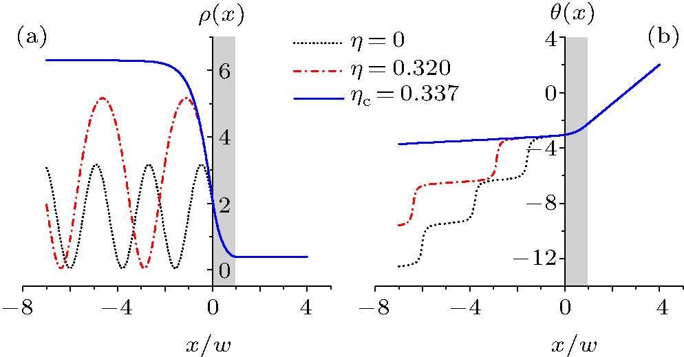 | Fig. 1. (a) Density ρ (x) and (b) phase θ (x) plotted for V = 3, w = 1, α = α 0 = 1.108, and C = C0 = 0.392 (kept 3 digits after the decimal point) with different η . The gray area indicates the region of the rectangular barrier. |
By increasing the nonlinearity to a critical value η c, a step-like density solution is obtained (the blue solid line in Fig. 1). And no solutions can be found by further increasing the nonlinearity (η > η c) for given C0 and α 0. When η = η c, the parameter m1 in Eq. (7) goes to 1 and the upstream density solution is reduced to ρ 1(x) = A + (2k2/η c) tanh2(kx + δ ). It can be proved that its asymptotic value at x → − ∞ is nothing but ρ 1(− ∞ ) = ρ sub (Eq. (12)) by combining m1 = 1 and the expression of the chemical potential μ 1. This means that the step-like density solution has the following property: its velocity is subsonic in the upstream, while supersonic in the downstream. Due to this velocity property, this kind of step-like density solution is also suggested to mimic the sonic black hole horizons in Refs. [18], [23], and [24].
This kind of solution has been obtained by numerical integration calculations in Refs. [20] and [28]. However in Ref. [20], the step-like density solution appears when the width of the barrier is increased to a critical value instead of the nonlinearity; and in Ref. [20], it is an asymptotic result of the time evolution of a steady subsonic density solution obtained with a supercritical injection velocity. According to our density solution (Eq. (7)), we can analytically find that the critical condition for the step-like density solution is m1(V, w, η , C, α ) = 1. So the critical nonlinearity plays as important a role as the critical width of the barrier.
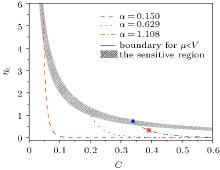
Considering m1 = 1 (at η = η c) and solving the matching conditions (8) by modifying the values of C for different α , we can find the relation of the critical nonlinearity η c with C (Fig. 2). The maximum critical nonlinearity is determined by μ = V (the black solid line in Fig. 2) for various current α . Usually, the maximum critical nonlinearity with a large current α is smaller than that with a small current. While, for a given C, a larger current allows a relatively larger critical nonlinearity (see the dotted or dashed lines in Fig. 2). As an example, the critical nonlinearity η c is marked as a red star in Fig. 2 for α = α 0 = 1.108 and C = C0 = 0.392, which is considered in Fig. 1 (the blue solid line). The gray region in Fig. 2 will be discussed in the following.
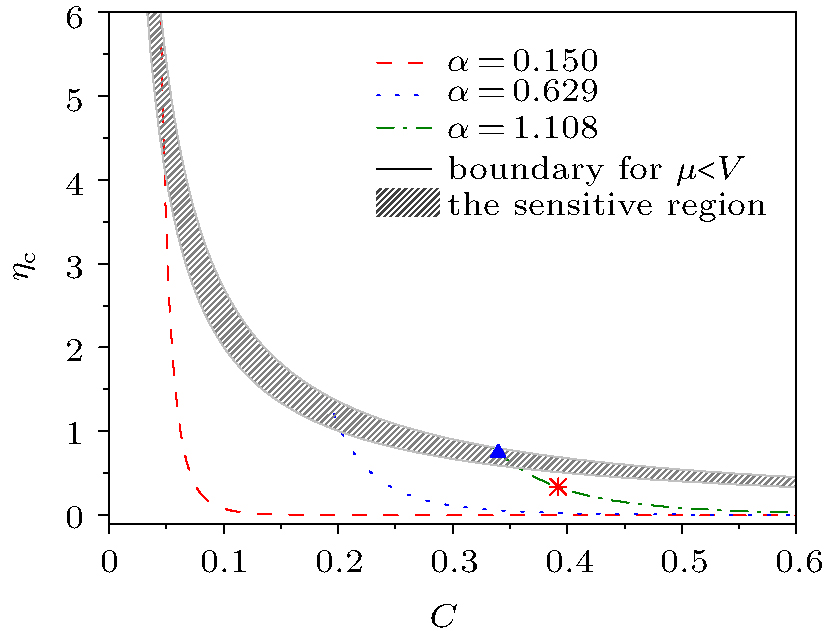 | Fig. 2. The critical nonlinearity η c as a function of C for different α , where V = 3 and w = 1. |
Since increasing the nonlinearity simultaneously enhances the repulsive nonlinear interaction, the chemical potential is increased too. To further explore the relation of the allowed nonlinearity with the chemical potential, equation (8) is also solved following the above procedure, except keeping the values of α = α 0 and μ . The allowed range of the nonlinearity for a given chemical potential is enlarged with increasing chemical potential. Once again, the critical nonlinearity (shown as the red dotted line in Fig. 3), as a boundary of the allowed nonlinearity, is found for the given chemical potential. Above the boundary, we do not find any solution for the nonlinear tunneling problem. The solid line in the inset shows the calculation details. The chemical potential μ is increased in a small step to enlarge the nonlinearity η .
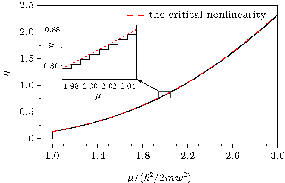 | Fig. 3. The nonlinearity η is plotted against μ for V = 3, w = 1, and α = α 0 = 0.384. The starting point from the linear tunneling is μ 0 = 1 and η = 0. |
Finally to investigate the stability of the step-like density solution at the critical nonlinearity η c, its time evolution, governed by Eq. (1), is numerically investigated with the help of the split-operator method.[29– 32] A ± 0.5% white position-dependent noise is added into the initial step-like solution. Two examples are shown in Fig. 4. It is easy to read that the long time evolution of the step-like density solution has good stability in Fig. 4(a) with the data of the blue solid line in Fig. 1 and the red star in Fig. 2, since there is no dramatical modification of the density solution after the long time evolution. While a dramatic modification can be found when t > 150 in Fig. 4(b), where the step-like density solution is for α = 1.108, C = 0.340, and η c = 0.743, (see the blue triangle in the gray region of Fig. 2). Many density solutions, whose parameters lie in the gray region of Fig. 2, show a similar evolution as that in Fig. 4(b). The reason may be that the chemical potential is very close to the height of the barrier in this region, and the density solutions are more sensitive to the parameters, such as the barrier position. But the rectangular barrier position is hard to describe accurately during the discretization of the position in numerical calculation. We think that the step-like solution is stable, although some examples, with parameters in the sensitive region of Fig. 2, fail in the simulations.
 | Fig. 4. The time evolutions of the step-like solutions. The initial small perturbation is added to the step-like density solution of (a) α = 1.108, C = 0.392, η c = 0.337; and (b) α = 1.108, C = 0.340, η c = 0.743. |
We have investigated nonlinear tunneling by analytically solving the GPE with a strong rectangular barrier. The properties of the nonlinear tunneling solutions, which can be reduced to the linear one, are explored. Only the supersonic solution in the downstream has a linear counterpart in the sense that it can be reduced to the linear one. There is a critical nonlinearity η c above which no tunneling solutions could be found from Eq. (8). Furthermore, the density solution has a step-like structure for η = η c. The maximum value of the critical nonlinearity is determined by μ = V for given α and C. The allowed range of the nonlinearity for given μ and α is enlarged with increasing chemical potential μ , and its boundary coincides with the critical nonlinearity. The step-like density solution at the critical nonlinearity η c has good stability against small perturbations. Our work may provide an additional way to create the step-like density, which has been suggested to mimic the sonic black hole horizon.[18, 23, 24]
We would like to thank Augusto Smerzi for his intriguing discussions.
| 1 |
|
| 2 |
|
| 3 |
|
| 4 |
|
| 5 |
|
| 6 |
|
| 7 |
|
| 8 |
|
| 9 |
|
| 10 |
|
| 11 |
|
| 12 |
|
| 13 |
|
| 14 |
|
| 15 |
|
| 16 |
|
| 17 |
|
| 18 |
|
| 19 |
|
| 20 |
|
| 21 |
|
| 22 |
|
| 23 |
|
| 24 |
|
| 25 |
|
| 26 |
|
| 27 |
|
| 28 |
|
| 29 |
|
| 30 |
|
| 31 |
|
| 32 |
|