†Corresponding author. E-mail: jinyf@bit.edu.cn
*Project supported by the National Natural Science Foundation of China (Grant No. 11272051).
In this paper, we investigate the solution moment stability for a Harrison-type predator–prey model with parametric dichotomous noises. Using the Shapiro–Loginov formula, the equations for the first-order and second-order moments are obtained and the corresponding stable conditions are given. It is found that the solution moment stability depends on the noise intensity and correlation time of noise. The first-order and second-order moments become unstable with the decrease of correlation time. That is, the dichotomous noise can improve the solution moment stability with respect to Gaussian white noise. Finally, some numerical results are presented to verify the theoretical analyses.
The interaction between the species and their natural environments has been extensively studied over the past decades.[1– 14] The predator– prey interaction is a basic structure in population dynamics and can be explored according to the mathematical model. In recent years, some theories of functional response have been developed to understand the complex dynamics of the predator– prey model. The functional response in a predator– prey model is the average number of preys killed per individual predator per unit time. Different types of functional responses, for example, Holling types I, II, III function, [6, 7] ratio-dependent functional response, [8, 9] and Beddington– DeAngelis function, [10, 11] can describe different kinds of species in population dynamics. In this paper, we consider a Harrison-type functional response, [12– 14] which describes a reduction in the predation rate at high predator densities due to mutual interference among the predators during food searching. The Harrison-type functional response predator– prey model is governed by the following equations:

where N = N(t) and P = P(t) describe the prey and predator population at time t, respectively, a is the natural growth rate of prey and a / b is the environmental carrying capacity, d is the natural death rate of the predator, c, m, and k denote the capturing rate, half capturing saturation constant, and conversion rate, respectively. All these parameters are positive.
In practice, numerous ecosystems are associated with random fluctuating environment or environmental noise, which can be modeled by using stochastic differential equations.[15– 21] May[15] pointed out that the birth rate, carrying capacity, competition coefficients, and other parameters involved in the ecosystem exhibit random fluctuations to a greater or lesser extent due to environmental noise. Mao[16] proved that noise can not only have a destabilizing effect but also have a stabilizing effect in the control theory. Saha and Banerjee[18] studied the exponential mean square stability of the interior equilibrium point for the delayed predator– prey model in the presence of parametric white and colored noises. Sun et al., [20] and Li and Jin[21] investigated the effect of colored noise on the pattern formation of a spatial predator– prey model. However, most of the above-mentioned papers are concerned with Gaussian white noise or the Ornstein– Uhlenbeck process. The dichotomous noise or random telegraph signal finds wide application in model building because of the simplicity of the two-state process.[22– 28] Meanwhile, the dichotomous noise is a better representation of real noise than the widely used Guassian white noise[27] and can be used to describe natural colored fluctuations. In this paper, we use the dichotomous noise to model the environmental noise in a predator– prey model and explore the effect of dichotomous noise on the stability of solution moment.
The rest of this paper is organized as follows. In Section 2, a Harrison-type functional response predator– prey model with parametric dichotomous noise is presented. In Section 3, the equations of solution moments and the corresponding moment stable conditions are obtained. In Section 4 some numerical simulations are provided to verify the theoretical results. Conclusions are summarized in Section 5.
Considering the effect of the environmental noise on model (1), we obtain the following equations:

where ξ i(t) (i = 1, 2) are the uncorrelated dichotomous noises, namely a kind of two-state random process, their means are both zero and correlation functions described as follows:

where σ i(i = 1, 2) are the noise intensities and τ is the correlation time of noises. Here ξ i(t) (i = 1, 2) take two values. For example,

where μ 1 is the transition rate of ξ 1(t) from M1 to − M2, μ 2 is the reverse rate, μ 3 is the transition rate of ξ 2(t) from M3 to − M4, μ 4 is the transition rate of ξ 2(t) from − M4 to M3, Δ 1 and Δ 2 denote the asymmetries of the dichotomous noises ξ i(t) (i = 1, 2) respectively. When Δ 1 = Δ 2 = 0, ξ i(t) (i = 1, 2) describe the symmetric dichotomous noises.
When λ = τ − 1 → ∞ , equation (3) degenerates to the Gaussian white noise with zero mean and correlation functions are

where Di(i = 1, 2) are the noise intensities of Gaussian white noise.
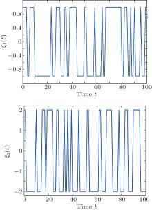
In Fig. 1, we use the method of acceptance– rejection to realize the stochastic processes for the dichotomous noises ξ i(t) (i = 1, 2).[23, 25, 26]
It is seen that the deterministic model of Eq. (1) has three equilibria as follows:

where

When ak > bd, the interior equilibrium E* is locally asymptotically stable.[14]
In this section, we consider the moment stability of the interior equilibrium E* and study the effects of dichotomous noises on the stability of system solution moment. Introducing a small perturbation (u, v) and assuming that N = N* + u, P = P* + v, we obtain the linearization of Eq. (2) as follows:

where

and ξ i(t) (i = 1, 2) defined by Eq. (4). For simplicity, we consider only the symmetric dichotomous noises in the following analysis.
Taking an average on Eq. (6), the first-order moment equations are obtained as follows:


Using the Shapiro– Loginov formula, [29] the following equality is obtained:

Multiplying Eq. (6) by ξ 1(t) and taking the average, then combining with Eq. (7), one has

Similarly, the following equations are obtained


The above linear differential equations (7)– (13) can be rewritten in the state space form as follows:

where state vector X = [ 〈 u〉 〈 v〉 〈 ξ 1u〉 〈 ξ 2v〉 〈 ξ 1v〉 〈 ξ 2u〉 ] T, the expression of system matrix A is given in Appendix A.
The corresponding characteristic equation of Eq. (14) is given as

where the expressions of coefficients ai(i = 60, … , 6) can be found in Appendix A.
According to the Routh– Hurwitz criterion, the solutions of Eq. (14) are stable if the following conditions are satisfied:

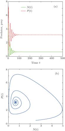
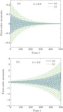
In order to show the stable region of the first-order moment, we choose the parameters to be a = 1.5, b = 0.1, c = 0.6, d = 0.2, k = 0.4, m = 0.1, and the initial conditions (N0, P0) = (1.5, 0.5). In Fig. 2, we plot the time histories and phase portrait for model (1) and find that the interior equilibrium E* = (0.65707235, 3.141447) is globally asymptotically stable. In Fig. 3(a), the stability boundary for the first-order moment is plotted in the (σ 1, σ 2) plane according to condition (16). When (σ 1, σ 2) falls into the below region bounded by the curve, the first-order moment of perturbation is stable as shown in Fig. 3(b). Otherwise, the corresponding first-order moment of perturbation is unstable as plotted in Fig. 3(c). Figure 4 shows the time histories of the first-order moment with different correlation times of noises. It is seen that the first-order moment of perturbation converges to zero and the first-order moment of the interior equilibrium is stable for λ = τ − 1 = 0.8 (see Fig. 4(a)). Figure 4(b) shows that the first-order moment of perturbation is divergent and the first-order moment of the interior equilibrium is unstable for λ = τ − 1 = 2.0.
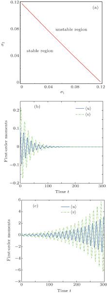 | Fig. 3. The first-order moment with λ = 5: (a) stable region; (b) time histories for σ 1 = 0.02, and σ 2 = 0.03; (c) time histories for σ 1 = 0.08, and σ 2 = 0.06. |
Using the Shapiro– Loginov formula, the following differential equations for the second-order moment are obtained;

where

the expression of system matrix B is given in Appendix B.
The corresponding characteristic equation of Eq. (17) can be obtained as

where the details of coefficients bi (i = 0, 1, … , 9) can be found in Appendix B.
Using the Routh– Hurwitz criterion, the stable conditions of Eq. (18) are derived as follows:

In order to check the stable conditions (19), the second-order moments of perturbation for different values of λ are plotted in Fig. 5. In Fig. 5(a), the second-order moment of perturbation is divergent for λ = τ − 1 = 3.0. Then, the correlation time of noise is increased to λ = τ − 1 = 0.2 in Fig. 5(b), the second-order moment of perturbation tends to zero. In Fig. 6,
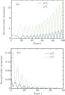 | Fig. 5. The second-order moments with the noise intensities σ 1 = 0.02, σ 2 = 0.03 and the different correlation times: (a) λ = τ − 1 = 3.0 and (b) λ = τ − 1 = 0.2. |
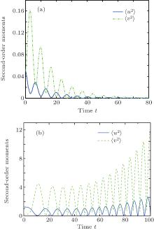 | Fig. 6. The second-order moments with λ = τ − 1 = 0.5 and different noise intensities: (a) σ 1 = 0.02, σ 2 = 0.01; (b) σ 1 = 0.03, σ 2 = 0.06. |
we fix the correlation time τ = λ − 1 = 2 and plot the second-order moments of perturbation with different noise intensities. It is seen that the second-order moment becomes unstable with the increase of noise intensity (see Figs. 6(a) and 6(b)).
In order to check the above theoretical results, we give some numerical results of model (2) in this section. In Figs. 7 and 8, we choose the same values of system parameters as those in Figs. 5 and 6. Figure 7 shows the plots of the evolutionary predator and prey populations for fixed noise intensities σ 1 = 0.02 and σ 2 = 0.03 and different correlation times. It is seen that the predator and prey populations oscillate around the interior equilibrium E* = (0.65707235, 3.141447) for λ = τ − 1 = 0.2 in Fig. 7(a). When the correlation time of noise is chosen as λ = τ − 1 = 3.0 in Fig. 7(b), the amplitudes of the predator and prey populations increase obviously and the interior equilibrium is unstable, which is consistent with the result shown in Fig. 5. In other words, the stability of solution moment can be improved by increasing the correlation time of noise. Figure 8 shows the time histories of the predator and prey populations for fixed correlation time λ = τ − 1 = 0.5 and different noise intensities. When the noise intensities are chosen as σ 1 = 0.02, σ 2 = 0.01, the amplitudes of predator and prey populations fluctuate around the interior equilibrium (see Fig. 8(a)). When the noise intensities increase to σ 1 = 0.03 and σ 2 = 0.06, the amplitudes of predator and prey populations become very big and fluctuate far from the interior equilibrium (see Fig. 8(b)). That is, the stability of solution moment can be destabilized by increasing the noise intensity, which is consistent with those obtained in Fig. 6. Therefore, it is shown that the dichotomous noise can improve the stability of system solution moment with respect to Gaussian white noise.
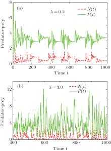 | Fig. 7. Time histories of model (1) with σ 1 = 0.02, σ 2 = 0.03 and different correlation times: (a) λ = τ − 1 = 0.2 and (b) λ = τ − 1 = 3.0. |
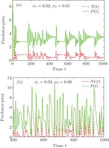 | Fig. 8. Time histories of model (1) with λ = τ − 1 = 0.5 and different noise intensities: (a) σ 1 = 0.02, and σ 2 = 0.01; (b) σ 1 = 0.03, σ 2 = 0.06. |
In this paper, we study the solution moment stability of a Harrison-type predator– prey model with parametric dichotomous noises. The equations of the first-order and second-order moments are derived and their stability conditions are obtained. It is found that the moment stability of the interior equilibrium does not change for sufficiently small random perturbation. When the noise intensity increases, the interior equilibrium becomes unstable. That is, the solution moment stability can be destabilized by a large random environmental perturbation. Furthermore, the interior equilibrium becomes unstable if the correlation time is sufficiently small. In other words, the dichotomous noise makes the interior equilibrium more stable than the Gaussian white noise. Considering the variability of environmental noises, more different types of noises (e.g. trichotomous noise, [30] Levy noise[31]) can be introduced into a predator– prey model. Meanwhile, the method used in this study can also be applied to the case of asymmetric dichotomous noises.
| 1 |
|
| 2 |
|
| 3 |
|
| 4 |
|
| 5 |
|
| 6 |
|
| 7 |
|
| 8 |
|
| 9 |
|
| 10 |
|
| 11 |
|
| 12 |
|
| 13 |
|
| 14 |
|
| 15 |
|
| 16 |
|
| 17 |
|
| 18 |
|
| 19 |
|
| 20 |
|
| 21 |
|
| 22 |
|
| 23 |
|
| 24 |
|
| 25 |
|
| 26 |
|
| 27 |
|
| 28 |
|
| 29 |
|
| 30 |
|
| 31 |
|


