


A cellular automata model of traffic flow with variable probability of randomization*
[Zheng Wei-Fana), b) , Zhang Ji-Yea)†  ]
]
]
|
|


†Corresponding author. E-mail: jyzhang@home.swjtu.edu.cn
*Project supported by the National Natural Science Foundation of China (Grant Nos. 11172247, 61273021, 61373009, and 61100118).
Research on the stochastic behavior of traffic flow is important to understand the intrinsic evolution rules of a traffic system. By introducing an interactional potential of vehicles into the randomization step, an improved cellular automata traffic flow model with variable probability of randomization is proposed in this paper. In the proposed model, the driver is affected by the interactional potential of vehicles before him, and his decision-making process is related to the interactional potential. Compared with the traditional cellular automata model, the modeling is more suitable for the driver’s random decision-making process based on the vehicle and traffic situations in front of him in actual traffic. From the improved model, the fundamental diagram (flow–density relationship) is obtained, and the detailed high-density traffic phenomenon is reproduced through numerical simulation.
Along with the increase of population and vehicles, the development of roads is difficult for satisfying the needs of vehicular traffic. The vehicular traffic modeling research has been an active area for many decades.[1, 2] To obtain the intrinsic evolution rules of the traffic system and methods for the management of traffic flow, many different approaches to model the behavior of the vehicular traffic system have been continuously studied. Since 1932, [3] many different models have been presented. There are several ways to distinguish these theories, e.g., microscopic[4, 5] vs. macroscopic[6, 7] and deterministic vs. stochastic. There are many deterministic traffic flow models, [8, 9] which mainly describe parameter fitting to simulate the concrete behavior of traffic flow.
The complex nonlinear phenomenon of traffic flow is dependent on the transition of variable traffic states. There are different traffic phases, such as free flow, synchronized flow, congested flow, and wide moving jam.[2] We could find the stable, meta-stable, and non-stable regions in the flow– density relationship diagram. Because of nonlinear characters of vehicular traffic, such as self-organization and high-density behavior above the critical density, it is hard to calculate the probability related to randomization when considering the effects of dynamically changed traffic states. It is difficult for the deterministic models to capture the effects of the variable behavior above the critical density because of its inability to describe the probability. Thus, many of these models have been condemned, [10, 11] and this results in an abundant improvement in the following research.[12, 13]
One of the classic methods to describe the random effects of traffic flow is cellular automata (CA) models, which were proposed by Nagel– Schreckenberg (NS model)[14] first. After that, a number of improvements have been proposed. In Refs. [15] and [16], the acceleration process was improved. In Refs. [17]– [19], the probability of randomization was reduced to a velocity function. In Ref. [20], the effects of brake lights were investigated. Recently, to avoid collisions, the effects of the safety probability were investigated by Mou et al.[21] The effects of random probability to the CA traffic flow model’ s slowdown behavior were obtained by Ding et al.[22] By introducing the remember parameter, a driver could properly adjust the random probability according to historic experience and current traffic situations in his model. These effects were considered to be able to forecast the chaotic behavior of the microscopic traffic, such as the congestion model and heavy synchronized flow. The model of mixed vehicles with fast and slow speeds was studied by Bentaleb et al.[23] The results of the weighted mean velocity feedback policy were investigated by Xiang et al.[24] A continuous cellular automata traffic flow with fuzzy logic was proposed by Yeldan et al.[25, 26]
The CA models mentioned above usually adopt the stationary slowdown probability. Most of them are still the deterministic models with added random noise, probability, and preference.[27, 28] It is hard to capture the variable behavior above the critical density. The random probability was considered by Ding et al.[22] The driver’ s remember parameter was introduced to improve the slowdown probability in his model. However, it is a pity for his model to adopt a stationary probability in the deceleration process. To describe the random phenomenon of high-density traffic flow, Alexandros Sopasakis and Markos A. Katsoulakis[27, 28] proposed a stochastic traffic flow model (AM model) that is based on the Arrhenius dynamic method, and the state of traffic is described by the results of the random driving system. Vehicles advance based on the interactional potential of the traffic situations. There, the interactional potential is the look-ahead potential that can be felt by the driver from the situation of the traffic in the length of the look-ahead parameter. The AM model reproduced the high-density traffic behavior by a numerical simulation. It was applied to a multi-lane traffic system in Ref. [29] and was extended to a non-lattice system in Ref. [30]. The statistical properties of the AM model were studied in Ref. [31].
The method of the AM model proposes a mechanism to describe the random decision-making process according to traffic situations such as vehicles and road situations before the driver. The mechanism complements the shortcomings of the CA model’ s random slowdown process described by stationary probability. In actual traffic, the decision-making process is randomly changed along with the traffic situation before the driver. The AM model could simulate the variable high-density traffic behavior. Inspired by the AM modeling process, in this paper, by using the dynamically changed probability to replace the classical NS model’ s stationary probability in the randomization step, we propose a new cellular automata traffic flow model with variable probability (VP model). From the new model, the fundamental diagram is obtained, and the complex high-density traffic phenomenon is reproduced by numerical simulation.
The remainder of this paper is organized as follows. Section 2 discusses the modeling process, Section 3 reviews the numerical simulation and gives the results, and Section 4 summarizes the primary conclusions and discussion of this study.
In this section, we will describe the model improved from the typical CA models. In the NS model, [14] a single-lane highway is divided into many discrete cell lattices at a typical space, which is the physics space occupied by vehicles in high-density traffic flow. Each cell can be occupied by at most one vehicle or is empty. The length of each cell is set as 7.5 m, approximately 22 feet. The maximal expected safety speed is vmax = 5 cells per second, and the velocity of each vehicle can take integer values between 0 and 5. There are four step movements in the CA model’ s rule set, including the acceleration, deceleration, randomization with probability p, and the vehicle’ s position update.
The CA models in existence usually adopt the stationary randomization probability. Few revised models consider that the decelerate process is not fixed in the randomization process in actual traffic. In fact, the driver’ s decision-making process is determined by the traffic situations before him, including each vehicle’ s dynamic changed distance and speed. So, the slowdown probability of randomization is randomly changed with the traffic situations before the driver. Referring to the mechanism describing the probability of randomization in the AM model, [27– 31] the dynamic changed transition rate is adopted to replace the stationary slowdown randomization probability in the randomization step. The modeling process is as follows.
A one-dimensional highway road is divided into N cells, L = {1, 2, … , N}. On each of the cell sites x ∈ L, we define an order parameter σ (x),

Similar to the Arrhenius dynamics for Ising systems, [32] the interactional potential has the form

where J denotes an anisotropic short range inter vehicle interactional potential of the form

Here γ = 1/(2l + 1) is a parameter prescribing the range of microscopic interactions and l denotes the potential radius. Specifically, we let V : R → R and set V(r) = 0 when r ∈ R− and r ≥ 1. In the simulations, we choose a simple constant potential of the form

where J0 is a parameter of interactional potential strength, and its sign implies attractive, repulsive, or no-interaction. In our simulations, we implement J0 > 0, which implies that vehicles are attracted by the empty space in front of them.
Vehicles are assumed to move from left to right. Vehicles cannot move backward in traffic, and only one vehicle is allowed to occupy one cell at a time. Periodic boundary conditions are imposed so that σ (mN + x) = σ (x) for any x ∈ L and any integer m.
The state transitions of σ (x) are the mechanism for modeling vehicle movement. They obey the rules of an exclusion process:[33] two cells exchange values in each transition, and vehicles may not move into occupied cells. The vehicles are only allowed to move into cells to the right. Thus, the only possible state transition of cells is of the form

In general, the transition rate at which a process will do this in spin-exchange Arrhenius dynamics[28] is
where the parameters are c0 = 1/τ 0, with τ 0 as the characteristic or relaxation time for the process. Thus, the state transition of cells between sites x and y during the time interval [t, t + Δ t] occurs with probability

The term exp [− U(x, σ )] plays the role of a slowdown factor when the forward vehicle density is high. Based on this probability, the driver’ s moving (or not) decisions take place.
The modeling process described above could be formulated as a continuous-time Markov chain, and the generator of this process can be computed explicitly. As discussed in Refs. [27] and [31], a closure is found under two assumptions.
Assumption 1 The look-ahead interactions are weak.
Assumption 2 The probability measure on σ (x) is approximately a product measure.
A coarse grain model and a traffic stream formulation equivalent to the Burgers equation could be derived by first computing the action of the generator on the finite test function, which in the simplest case of no interactions (J0 = 0) and corresponds to the well-known Lighthill– Whitham flux.[6]
From formulas (2) and (3), and r > 0 in the potential radius, when the interactional strength J(x, y) takes the form of constant J0, the potential function could be revised as

where parameter Q is the number of vehicles to the right of site x, which affects the velocity of the vehicle at site x. Namely, Q is the look-ahead length of the vehicle at site x. Thus, the state transition probability of cells is changed as
From the above consequence, the CA model’ s stationary slowdown probability in the randomization step could be replaced by the state transition probability of cells. Thus, the improved cellular automata model of traffic flow with variable probability of randomization is obtained and includes four steps as follows:
Step 1 Acceleration process If vi < vmax, the speed of the i-th vehicle is increased by one unit. The rule is given as vi (t + 1) → min (vi (t) + 1, vmax).
Step 2 Deceleration process If gapi < vi, the speed of the i-th vehicle is reduced to gapi − 1. The rule is given as vi (t + 1) → min (vi (t) + 1, gapi − 1), where gapi = xi − xi − 1.
Step 3 Randomization slowdown process with variable probability In this step, if vk > 0, the speed of the k-th vehicle is decreased randomly by one unit with the dynamic changed probability. Calculate the look-ahead potential and the state transition rate of cells at site x by formulas (7) and (8). If σ k (t) = = 1 and σ k + 1 (t) = = 0, then a random number p between [0, 1] is generated. Additionally, if the random number p is less than the state transition rate, i.e., p < c0 exp (− J0Uk (x, σ ))Δ t, then the k-th vehicle at site x could move forward and would not need to reduce its speed. The rules are given as σ k (t + Δ t) = 0, σ k + 1 (t + Δ t) = 1, and vk + 1 (t + 1) → vk (t + 1). Otherwise, the speed of the k-th vehicle at site x will be reduced by one unit with probability c0 exp (− J0Uk (x, σ ))Δ t. The rule is given as vk (t + 1) → max (vk (t + 1) − 1, 0).
Input: The length of the highway L and the number of cells N, maximal velocity vmax, look-ahead length Q, time t, time step δ t, interactional potential strength J0, and the initial value of the order parameter σ k (t).
Initialization: Vehicles enter the road with a certain distribution.
Loop: Calculating the gaps: gapi (t) = xi (t) − xi − 1 (t);
Acceleration: vi (t + 1) → min (vi (t) + 1, vmax);
Deceleration: vi (t + 1) → min (vi (t) + 1, gapi − 1);
Randomization slowdown:
for k = 1: N do
if σ k (t) = = 1 and σ k + 1 (t) = = 0 then

p = rand();
if p < c0 exp (− J0Uk (x, σ ))δ t then
σ k (t + δ t) = 0, σ k + 1 (t + δ t) = 1, vk + 1 (t + 1) → vk (t + 1);
else vk + 1 (t + 1) → max (vk (t + 1) − 1, 0);
end if
end if
end for
Vehicle position update: xi (t + 1) → xi (t) + vi (t + 1).
Step 4 Vehicle position update process After three steps, the new position of each vehicle can be determined by using the current velocity and the current position. The rule is given as xi (t + 1) → xi (t) + vi (t + 1).
From the above steps, we can obtain the evolution algorithm of our one-lane CA model as follows.
Matlab is used to simulate the one-lane traffic flow system. In our simulation, the number of cells is N = 60, and the length of each cell is 7.5 m, which is approximately 22 feet. Then, the total length of the highway is 60 × 7.5 = 450 m. The maximal expected safety speed is 135 km/h, i.e., vmax = 5 cells per second. Other parameters are c0 = 1/τ 0 = 1/0.23 = 4.3478.[27] The vehicles only move forward or stop. The speed of each vehicle is non-negative, namely, each vehicle cannot move backward. The sampling frequency is 100, i.e., the time step is 0.01.
To simulate the actual highway, we take the open boundary conditions. Vehicles enter the cells from the left side of the road and leave the cells from the right side of the road. The probability of the initial distribution of vehicles in the cells is 0.5. The vehicles reach the first cell randomly and leave the last cell by a probability of 0.5. The density of each vehicle is calculated by using the instantaneous density, and the flux of the traffic is measured as the number of vehicles passing a detector at a given time interval. The results and discussion are presented as follows.
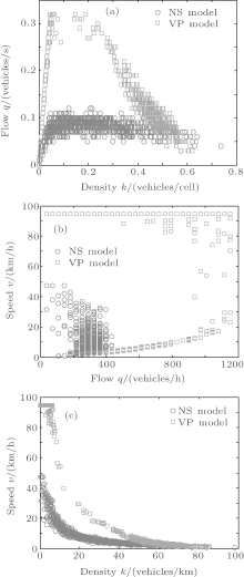
To compare the results of the NS model and VP model, the same type of curves for the two models are drawn in the same figure. The parameters of the VP model are Q = 2, C0 = 4.3478, J0 = 6, and vmax = 4. The slowdown probability of randomization in the NS model is 0.2. The total run time is 800 s. The simulation results of the flow– density, flow– speed, and density– speed relationships are presented in Fig. 1, and the curves of flow, density, and speed changing with time are presented in Fig. 2.
From Fig. 1(a), we can see that the areas of free flow, congested flow, and wide moving jam in the VP model are larger than those in the NS model. The critical density of traffic in the VP model is higher than that in the NS model, which is 0.12 vehicles per second in the NS model, and 0.33 vehicles per second in the VP model. As shown in Fig. 1(b), the maximal flow of traffic in the VP model is higher than that in the NS model, which is 450 vehicles per hour in the NS model, and 1200 vehicles per hour in the VP model. As shown in Fig. 1(c), the maximal speed of traffic in the VP model is higher than that in the NS model, which is 48 km/h in the NS model, and 95 km/h in the VP model.
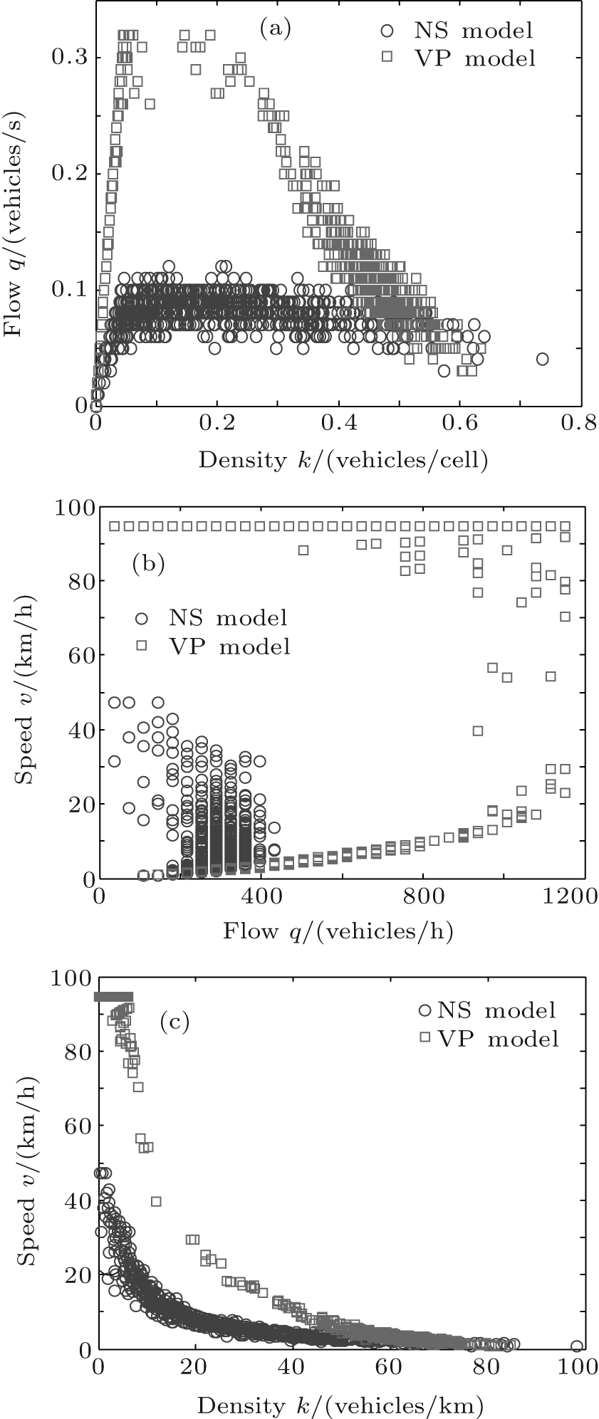 | Fig. 1. (a) Flow– density, (b) flow– speed, and (c) speed– density relationships. |
From Fig. 2(a), we can see that the maximal flux is approximately 0.08 vehicles per second, which occurs at the free flow after running 100 s in the NS model, and the maximal flux is approximately 0.32 vehicles per second, which occurs at the free flow after running 250 s in the VP model. As shown in Fig. 2(b), the maximal density of traffic is approximately 0.1 vehicles per cell in the NS model, while it is approximately 0.5 vehicles per cell in the VP model. From the curve shown in Fig. 2(c), we can obtain the same results for the maximal speed of traffic in the two models as shown in Fig. 1(c).
 | Fig. 2. (a) Flow– time, (b) density– time, and (c) speed– time diagrams. |
Figures 1 and 2 show that the VP model greatly improves the flux and density of the traffic system. This is mainly because in the VP model, the driver’ s deceleration decisions in the randomization slowdown step are randomly made according to the interaction potential of traffic situations before the driver rather than with the stationary slowdown probability. Thus, the decision-making process could avoid the needless decrease in speed of each vehicle due to the stationary slowdown probability. In this case, the interactional potential is small, and each vehicle does not need to decrease its speed in the VP model.
From Fig. 3, we can clearly observe the expected rarefaction wave on one side and the shock wave on the other side, which clearly displays the phenomenon of stop-and-go. Furthermore, the character of the wave’ s movement in the VP model is clearer than that in the NS model. The results presented here coincide well with in Ref. [27]
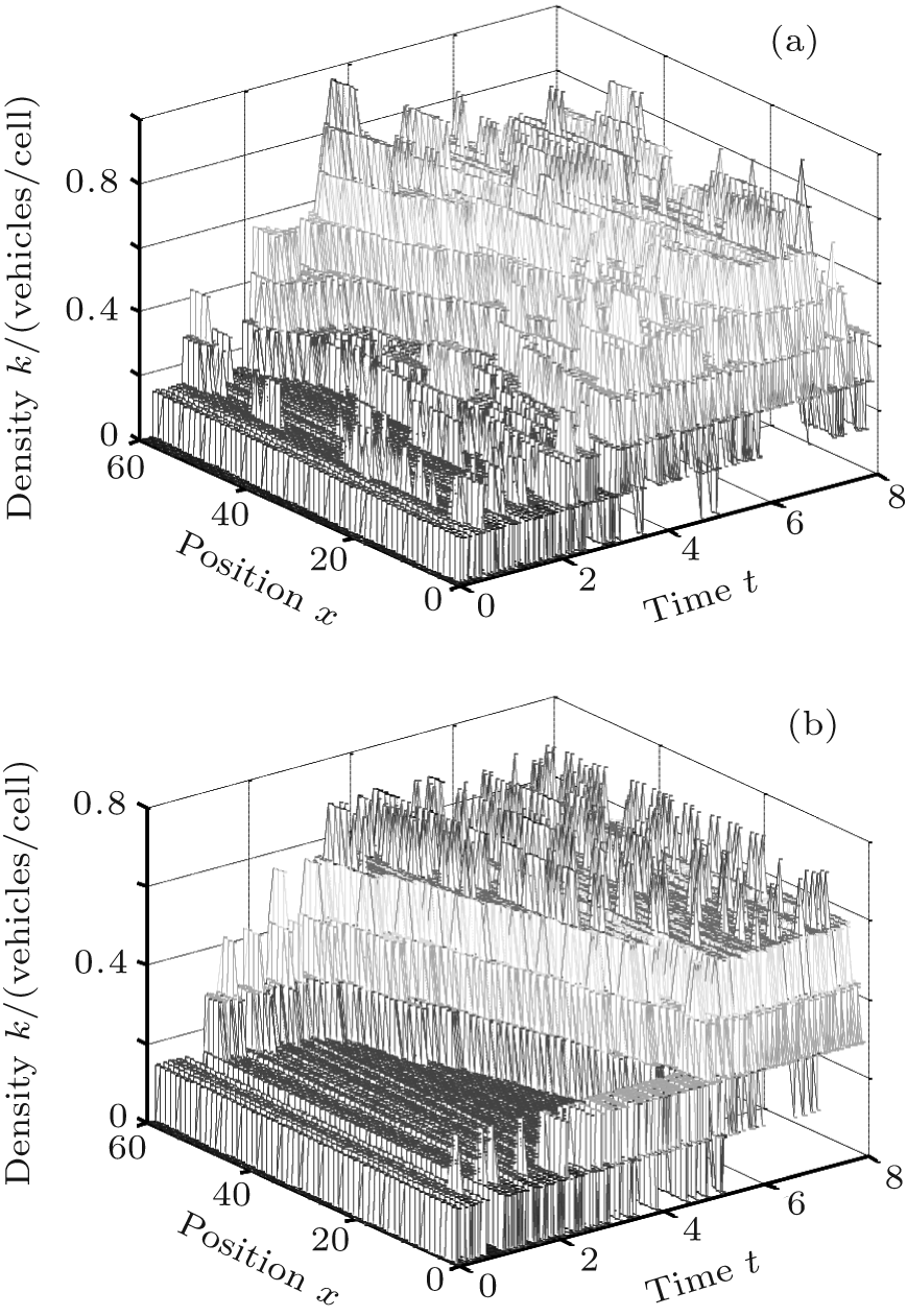 | Fig. 3. (a) The results evolved by the NS model, in which the decreased probability in the randomization step is 0.2, vmax = 4, and the total run time is 800 s. (b) The results evolved by the VP model, in which the interactional potential strength is J0 = 3, the look-ahead length is Q = 4, vmax = 4, and the total run time is 800 s. |
Under the fixed look-ahead length, we experiment with different values of the interactional potential strength. The simulation parameters are vmax = 4, J0 = 0, 2, 4, 6, 8, and the total run time is 800 s. The simulation results are presented in Fig. 4.
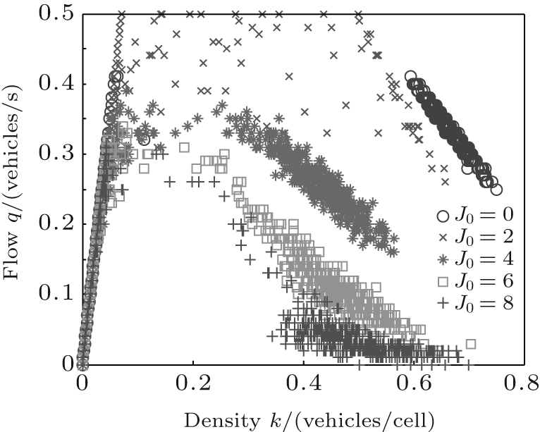 | Fig. 4. Comparison of the fundamental diagrams with Q = 2 and different J0. |
We note in Fig. 4 that the density– flow curve is convex at first and then gradually changes to concave and then is neither convex nor concave with the increase of J0. The results are in good agreement with Fig. 10 in Ref. [27]. The maximal flow and the critical density of traffic gradually decrease with the increase of J0.
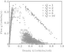
Under the fixed interactional potential strength, we experiment with different values of the look-ahead length. The simulation parameters are vmax = 4, Q = 1, 2, 4, 8, 16, and the total run time is 800 s. The simulation results are presented in Fig. 5.
 | Fig. 5. Comparison of the fundamental diagrams with J0 = 10 and different Q. |
We note in Fig. 5 that the density– flow curve is convex at first and then gradually changes to concave and is neither convex nor concave with the increase of Q. The results are in good agreement with Fig. 9 in Ref. [27]. The maximal flow and the critical density of traffic gradually decrease with the increase of Q.
Figures 4 and 5 show that in the low-density traffic cases, the density– flow curves are a superposition. From the results, we note that the variable probability in the VP model has a slight effect on the low-density traffic flow. This is mainly because in the low-density cases, traffic flow is nearly free flow; drivers can travel at their own desired speed and be infrequently affected by the vehicles in front of them. Therefore, there is nearly no interaction between the vehicles in low-density traffic.
Research on the stochastic behavior of traffic flow is important to understand the intrinsic evolution rules of the traffic system. In this paper, we have presented an improved cellular automata model for traffic flow, which could describe the stochastic behavior of high-density traffic flow. In the modeling process, the interactional potential is introduced to describe the interactional effects of vehicles before the driver. The stationary probability of the randomization step in the CA models is replaced by the variable probability related to this interactional potential. The interactional potential proposed in this paper is presented as a potential function, which is mainly related to three parameters: interactional potential strength J0, relaxation time τ 0, and look-ahead length Q. These parameters play an important role in describing the dynamics of the traffic state transition. Compared with the traditional cellular automata model, the modeling is more suitable for the driver’ s random decision-making process, which is based on the vehicle and traffic situations in front of him in actual traffic.
Subsequently, we compare the results of our new model with those of the NS model for a variety of parameters by using numerical experiments. From these experiments, we obtain the fundamental diagram, and the flow– speed and density– speed curves that display many of the observed traffic states, including phenomena such as stop-and-go. Furthermore, the effect of different interactional potential strength J0 and look-ahead length Q on traffic flow is investigated. The obtained results are in good agreement with those obtained empirically in the existing literatures.
There are two primary avenues of research that can be extended from our model. First, there is the need to explore the effects of all types of potential functions on traffic flow, including not only discrete functions but also continuous functions. These abundant potential functions could describe more detailed behavior of high-density traffic flow. The second is that we could extend the simulations presented here for one-lane traffic systems to multi-lane traffic systems.
| 1 |
|
| 2 |
|
| 3 |
|
| 4 |
|
| 5 |
|
| 6 |
|
| 7 |
|
| 8 |
|
| 9 |
|
| 10 |
|
| 11 |
|
| 12 |
|
| 13 |
|
| 14 |
|
| 15 |
|
| 16 |
|
| 17 |
|
| 18 |
|
| 19 |
|
| 20 |
|
| 21 |
|
| 22 |
|
| 23 |
|
| 24 |
|
| 25 |
|
| 26 |
|
| 27 |
|
| 28 |
|
| 29 |
|
| 30 |
|
| 31 |
|
| 32 |
|
| 33 |
|