

Cooling and trapping polar molecules in an electrostatic trap*
[Wang Zhen-Xia, Gu Zhen-Xing, Deng Lian-Zhong, Yin Jian-Ping† ]
]
]
|
|


†Corresponding author. E-mail: jpyin@phy.ecnu.edu.cn
*Project supported by the National Natural Science Foundation of China (Grant Nos. 10674047, 10804031, 10904037, 10974055, 11034002, and 11274114), the National Key Basic Research and Development Program of China (Grant Nos. 2006CB921604 and 2011CB921602), the Basic Key Program of Shanghai Municipality, China (Grant No. 07JC14017), and the Shanghai Leading Academic Discipline Project, China (Grant No. B408).
An electrostatic trap for polar molecules is proposed. Loading and trapping of polar molecules can be realized by applying different voltages to the two electrodes of the trap. For ND3 molecular beams centered at ∼10 m/s, a high loading efficiency of ∼67% can be obtained, as confirmed by our Monte Carlo simulations. The volume of our trap is as large as ∼3.6 cm3, suitable for study of the adiabatic cooling of trapped molecules. Our simulations indicate that trapped ND3 molecules can be cooled from ∼23.3 mK to 1.47 mK by reducing the trapping voltages on the electrodes from 50.0 kV to 1.00 kV.
The rich internal structure of cold molecules makes them ideal for study of phenomena like fundamental physical constants, [1, 2] cold collisions, [3, 4] cold chemistry, [5] quantum calculation, [6] etc. A variety of techniques have already been developed to trap cold molecules. In 2000, Meijer’ s group first confined ND3 molecules of weak-field-seeking states (WFS) in an electrostatic trap.[7] Later, they successfully loaded OH radicals[8] and metastable CO molecules[9] into a similar trap, respectively. In 2005, the Rempe group reported a continuously operated electrostatic trap, [10] and a packet of ND3 molecules was confined at a density of 108 cm− 3. Later, they demonstrated a microstructured box-like electric trap[11] where molecules can be stored for up to 60 s. By slowly expanding the trap volume, adiabatic cooling of trapped molecules can be realized. In 2007, our group described an electrostatic trap for cold molecules formed by a pair of parallel transparent electrodes and a ring electrode[12] as well as an electrostatic surface trap with a charged circular wire.[13] In the next few years, two other surface traps for cold polar molecules on a chip were presented, [14, 15] and loading efficiencies of 11.5% and 88% were obtained respectively. In 2013, we proposed an electrostatic trap for cold molecules with 3D optical access.[16] The electric field in the x direction of the trap is much weaker than those in the two other directions, resulting in an effective trap with shallow depth. In this paper, we propose a new electrostatic trap for cold molecules of WFS states with deeper depth and simpler structure. Also, it can be used to study the cooling effect of the trapped molecules.
In the following sections, the scheme of our proposed electrostatic trap is first presented together with the distribution of the electric field generated by the electrodes of the trap. Then, our Monte Carlo simulations for the processes of loading and confining ND3 molecules in the trap are reported. The cooling effect of trapped ND3 molecules is simulated as well. Some discussion and conclusions are presented at the end.
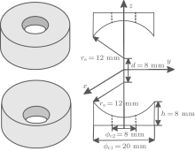
The electrostatic trap is composed of two charged electrodes. The two electrodes have the same geometry and are shaped in the following way: two 20-mm-in-diameter and 8-mm-in-height cylindrical electrodes are subtracted by part of a 12-mm-in-radius ball and then drilled through with an 8-mm-in-diameter hole in the center. The two pieces are placed with a face-to-face distance of 32 mm in the center, as shown in Fig. 1. The molecular beam moves into the trap along the direction of z.
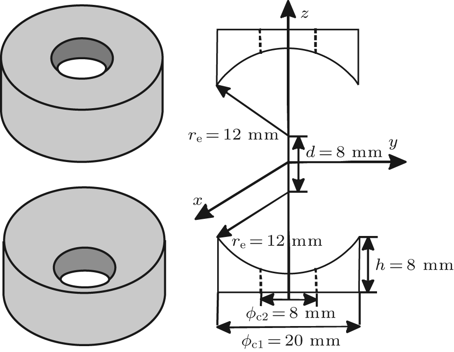 | Fig. 1. Schematic diagram of our proposed electrostatic trap. The two electrodes are the same in geometry and shaped in the following way: a 20-mm-in-diameter and 8-mm-in-height cylinder electrode is first subtracted by part of a 12-mm-in-radius ball and then drilled through by an 8-mm-in-diameter hole in the center. The two pieces are placed with a face-to-face distance of 32 mm in the center. The molecular beam is incident along the z axis. |
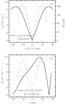
Using finite-element software, we calculated the electric field distribution of the trap when a high voltage U is applied to the two electrodes. The contour distributions of the electric field in the xy and yz planes are shown in Figs. 2(a) and 2(b), respectively, with the applied voltage U = 50.0 kV. We can find that the electric field is inhomogeneous with a minimum around the origin, a pattern which can be used to trap polar molecules in WFS states. Figure 3(a) shows the electric field distributions inside the trap along the x (or y) (solid line) and z axes (dashed line), respectively. The electric field distributions are the same in the x and y directions due to the cylindrical symmetry of the trap’ s structure. As we can see, the minima of the electric fields are zero at the center of trap. The maxima of the electric fields are nearly the same in all three directions and have a value of about ∼ 9 kV/cm. For ND3 molecules in the electrostatic field, the Stark potential is given by[17]
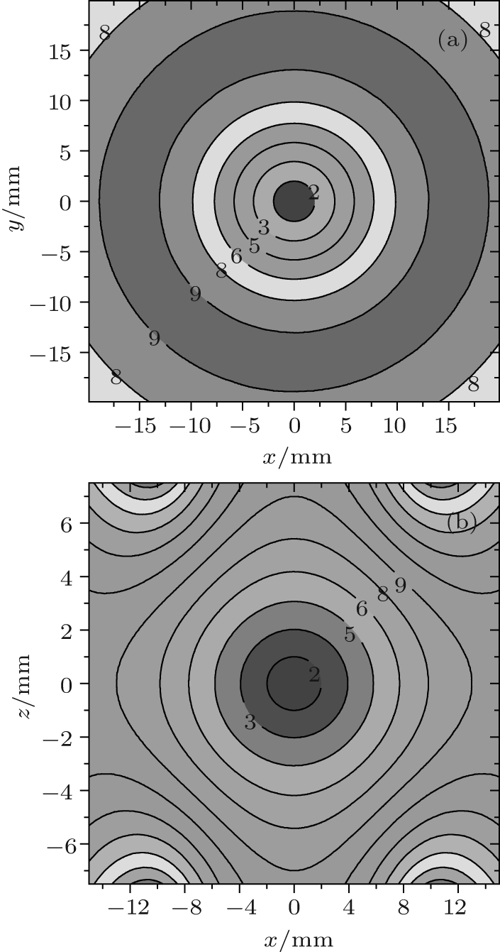 | Fig. 2. Contour distributions of the electrostatic field generated by the two electrodes in (a) xy and (b) xz planes with U = 50.0 kV. The labels in the figures are all in units of kV/cm. |
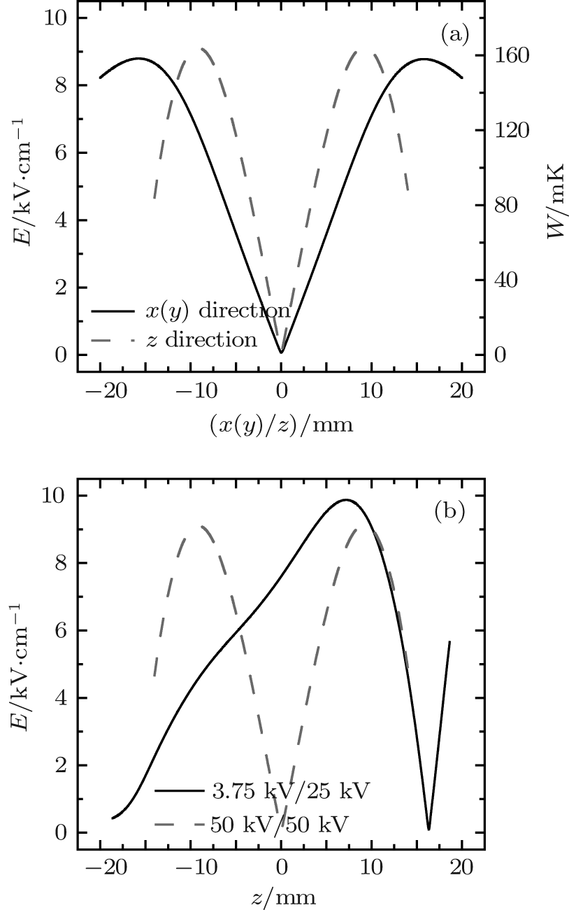 | Fig. 3. Spatial distributions of the electric field generated by the two electrodes. (a) The trapping configuration. The solid line stands for the distribution of electric field in the x (or y) direction and the dashed line shows that in the z direction. (b) The loading configuration. The solid line indicates the distribution in the z direction, i.e., the direction of incident molecular beam, and the dashed line is the same distribution of panel (a) and remains here for comparison only. |
where Winv is the inversion splitting, μ is the electric dipole moment of the molecule, J is the rotational quantum momentum, K is the projection of J on the molecule-fixed axis, and M is the projection of J on the space-fixed axis. We calculated the Stark potential of ND3 molecules of | J, K, M〉 = | 1, 1, − 1〉 state in the trapping field, and the results are shown by the right vertical axis in Fig. 3(a). We can see that the effective trap depth is about ∼ 160 mK, deep enough to trap molecules slowed by a Stark decelerator.
Molecules can be loaded into the trap through one of the holes in the electrodes. Our study shows that when the voltages are applied on the two electrodes, U1 and U2 are set to ∼ 3.75 kV and ∼ 25.0 kV respectively, the electric field is suitable for loading WFS molecules, as shown by Fig. 3(b). The incident ND3 molecules are first decelerated by the gradient force of the electric field when moving toward the trap center. The voltages U1 and U2 are both switched to ∼ 50.0 kV as the molecules reach the trap center. A 3D electrostatic trap is formed for those molecules whose kinetic energies are less than the trap depth.
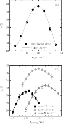
The dynamic processes of ND3 molecules being loaded into and trapped in the electrostatic well were numerically simulated using the Monte Carlo method. The simulated molecular number is N = 106, and the spatial and velocity profiles are both Gaussian, where the transverse and longitudinal spatial sizes are 6 mm and 12 mm, respectively, and the full-width at half maximum of the velocity profiles are 3 m/s in all three directions. Simulations were performed with molecular beams of different initial central velocities, and corresponding results are shown in Fig. 4(a). As we can see, the highest loading efficiency is achieved with an initial central velocity of ∼ 10 m/s. The dependence of the loading efficiency on the loading time was studied and some results are presented in Fig. 4(b). As we can see, there exists an optimal loading time for each initial central velocity, at which the maximal loading efficiency is obtained. For an initial central velocity of vz0 = 10 m/s, the optimal loading time is tloading = 3.0 ms, corresponding to a maximal loading efficiency of ∼ 67%. The reason is that if the loading time is shorter, many molecules have not yet reached the region of the trap center, and if the loading time is longer, molecules with lower velocities may be accelerated in the opposite direction, while molecules with higher velocities may pass through the potential barrier and accelerate away from the trap. Therefore, if the loading time is shorter or longer, the loading efficiency is not high.
 | Fig. 4. Dependences of the loading efficiency of cold ND3 molecules on both (a) the initial central velocity vz0 with Δ vx0 = Δ vy0 = Δ vz0 = 3 m/s and (b) the loading time tloading for different initial central velocity (vz0 = 9, 10, and 11 m/s) with U1 = 3.75 kV and U2 = 25.0 kV. The symbols are the simulated results with the solid lines being the fitted curves. |
Figure 5 shows the initial and final velocity distributions of the molecules before entering into and after being confined in the trap. As we can see, the velocity distribution of the trapped molecules is centered at zero. We estimated the temperature of the molecules in the trap. The temperatures of the trapped molecules are ∼ 16.6 mK in direction x (or y) and ∼ 36.5 mK in direction z, resulting in a 3D temperature of ∼ 23.3 mK. The volume of our trap is rather big and estimated to be about ∼ 3.6 cm3.
 | Fig. 5. The initial (circles) and final (five-pointed stars) velocity profiles of the simulated molecules in z (a), x (b), and y (c) directions. |
When the voltages applied to the electrodes decrease, the trap depth gets shallow. As the volume of molecules expands with the decreasing trap depth, the trapped molecules cool adiabatically. If the fast molecules have kinetic energies that are larger than the trap depth, they will escape and only slow molecules of low kinetic energies will remain, and thus the temperature of molecules in the trap will get low, very similar to the process of evaporative cooling.
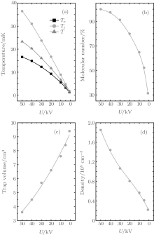
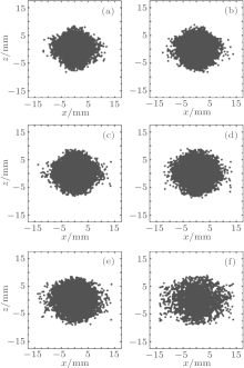
We numerically studied the trajectories of the molecules as the trapping voltages were gradually reduced from 50.0 kV to 1.00 kV. The temperature, the molecular number, the volume as well as the density of the trapped molecules were calculated for different voltages, and the results are shown in Fig. 6. The squares and circles in Fig. 6(a) represent the temperatures in x and z directions, respectively, while the triangles represent the 3D temperature of the molecules. When the trap voltage is reduced from 50.0 kV to 30.0 kV, the 3D temperature of molecules in the trap is cooled from ∼ 23.3 mK to ∼ 16.1 mK, and about 90% of the initial molecules still remain; the molecules are adiabatically cooled mainly. As the voltage is reduced further, the temperature of the molecules in the trap gets lower and lower; however, this occurs at the cost of the loss of a large number of molecules. When the voltage is reduced to 10.0 kV, the molecules begin to be lost dramatically. The temperature is reduced from 6.68 mK to 1.47 mK when the voltage decreases from 10.0 kV to 1.00 kV, and the cooling effect is dominated by evaporative cooling. With a final trapping voltage of 1.00 kV, a 3D molecular temperature of ∼ 1.47 mK is obtained and the corresponding number of molecules in the trap is about ∼ 31% of the initial number of molecules trapped. The number of the incident molecular beam is 106, with the loading efficiency of 67%, the density of the molecules before cooling is about 1.8 × 105 cm− 3 with the volume of 3.6 cm3. With the reduction of the trapping voltages, the number of the trapped molecules decreases, while the trap volume expands, resulting in a decrease of molecular density, and when the trapping voltage is 1.00 kV, the density of the cooled molecules is 2.2 × 104 cm− 3. Figure 7 shows the spatial distributions of the trapped molecules in the xz plane for different trapping voltages, and we can see the expansion of molecules visually as the voltage decreases.
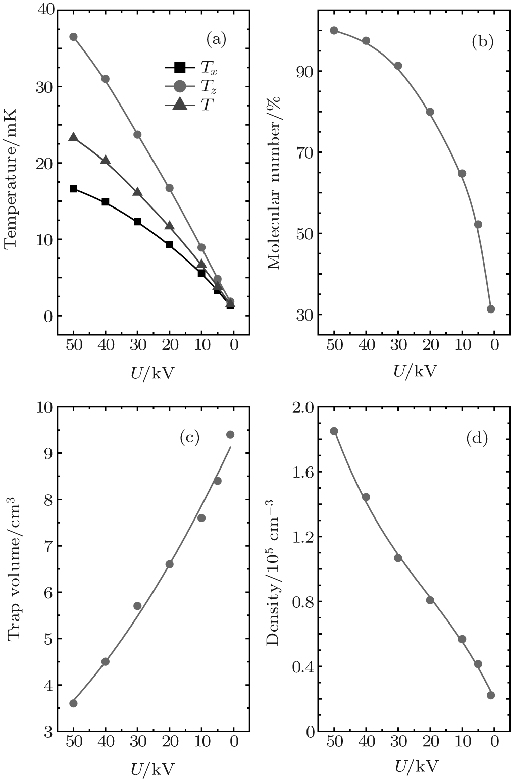 | Fig. 6. (a) The temperatures of the trapped molecules as a function of the trapping voltages. The squares stand for the temperature in x (or y) direction, the circles show the temperature in z direction, and the triangles indicate the 3D temperature of the trapped molecules. (b) The number of molecules in the trap relative to that of the molecules initially trapped. (c) The trap volume and (d) the density of the trapped molecules. |
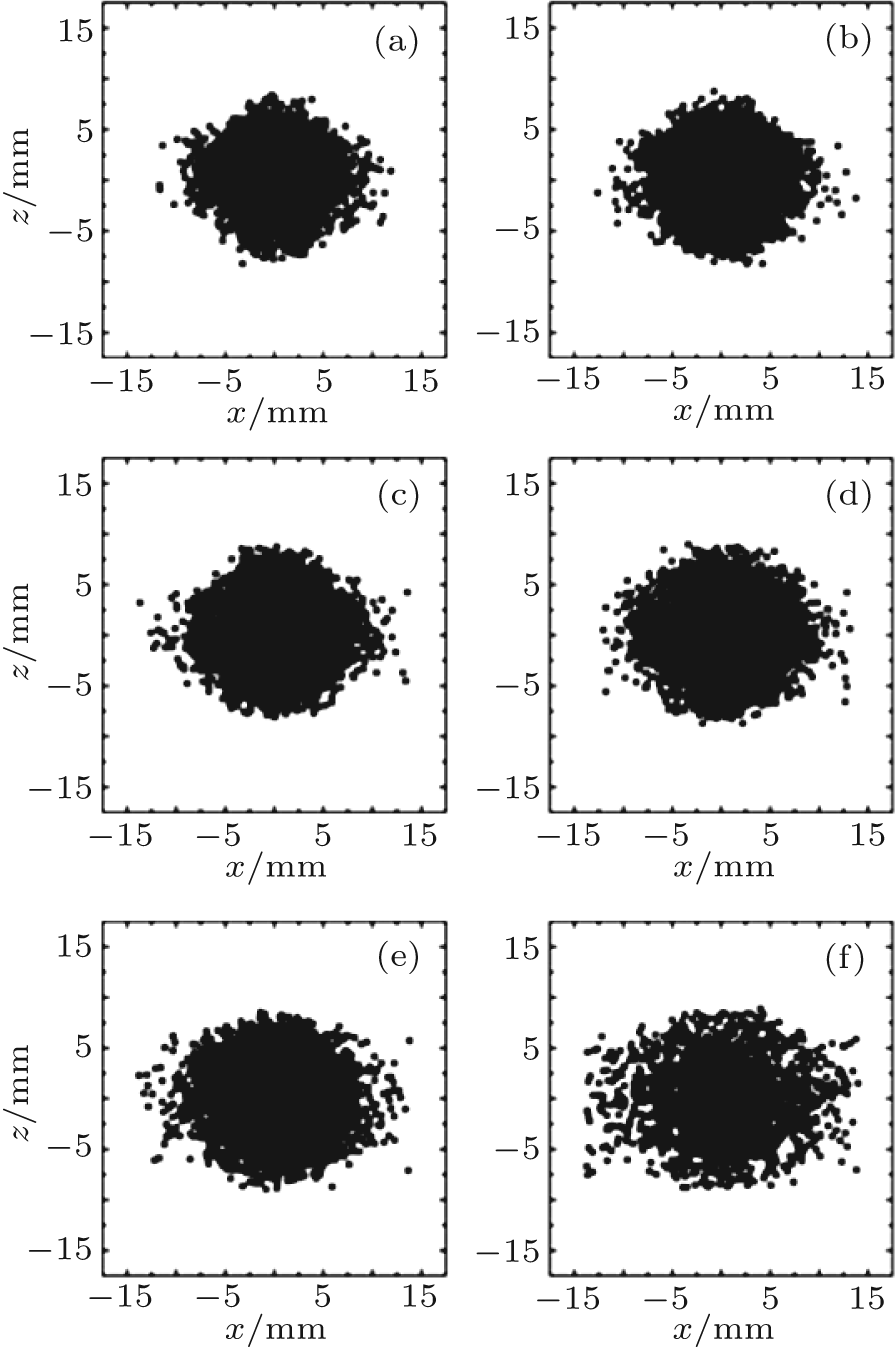 | Fig. 7. Spatial distribution of the trapped molecules in the xz plane as a function of the trapping voltages. Panels (a)– (f) stand for U = 50 kV, 40 kV, 30 kV, 20 kV, 10 kV, and 1 kV, respectively. |
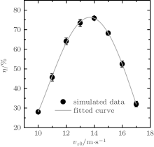
As the loading and trapping voltages increase, molecules of higher velocities can be accepted, and thus the optimal central velocity for loading increases. For instance, when U1 = 7.50 kV and U2 = 50.0 kV, the optimal central velocity for loading rises to ∼ 14 m/s, as shown in Fig. 8, and the corresponding loading efficiency reaches ∼ 76%. This means that a Stark decelerated molecular beam of a given velocity can be loaded into our trap efficiently by selecting appropriate voltages of the electrodes. However, the highest voltages available for loading and trapping are limited by the discharges between the energized electrodes, and these maximum voltages determine the upper limit of the initial central velocity of the molecules to be accepted.
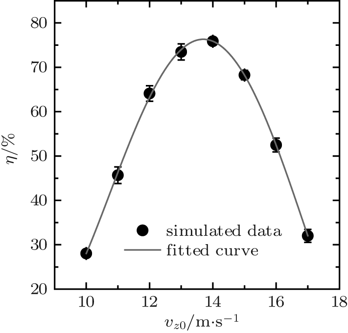 | Fig. 8. Dependence of the loading efficiency of cold ND3 molecules on the initial central velocity of vz0. Other parameters are: Δ vx0 = Δ vy0 = Δ vz0 = 3 m/s, U1 = 7.00 kV and U2 = 50.0 kV. The symbols are the simulated results with the solid line being the fitted curve. |
Compared with the trap described in Ref. [16], this trap has its own advantages. It is simpler in structure and can realize the loading and trapping of molecules without any additional electrodes. Furthermore, its effective trap depth is much deeper than that of the one discussed in Ref. [16], whose trap depth in the x direction is much shallower than those in the two other directions.
We have proposed a simple electrostatic trap for cold polar molecules with high loading efficiencies. The electric field distribution of the electrostatic well generated by the electrodes was numerically calculated. The dynamic motions of ND3 molecules being loaded into and trapped in the electrostatic well were simulated by a Monte Carlo method. Our study shows that Stark decelerated molecular beams can be efficiently loaded into our trap. For instance, when the loading voltages on the electrodes are U1 = 3.75 kV and U2 = 25.0 kV, molecular beams with an initial central velocity of 10 m/s are best suitable for loading the trap. With an optimal loading time of ∼ 3.0 ms, the loading efficiency is as high as ∼ 67%. The volume of the trap is estimated to be about ∼ 3.6 cm3. We have also studied the cooling effect of the molecules in the trap by changing the voltages applied on the electrodes. When the trapping voltages change from 50.0 kV to 1.00 kV, the temperature of the molecules in the trap is cooled from about ∼ 23.0 mK to ∼ 1.47 mK. If the loading voltages are increased to U1 = 7.00 kV and U2 = 50.0 kV, the optimal initial central velocity for loading will be increased to ∼ 14 m/s with the optimal loading efficiency rising up to ∼ 76%.
| 1 |
|
| 2 |
|
| 3 |
|
| 4 |
|
| 5 |
|
| 6 |
|
| 7 |
|
| 8 |
|
| 9 |
|
| 10 |
|
| 11 |
|
| 12 |
|
| 13 |
|
| 14 |
|
| 15 |
|
| 16 |
|
| 17 |
|