


Superfluidity of Bose—Einstein condensates in ultracold atomic gases*
[Zhu Qi-Zhonga) , Wu Biaoa), b), c)†  ]
]
]
|
|


†Corresponding author. E-mail: wubiao@pku.edu.cn
*Project supported by the National Basic Research Program of China (Grant Nos. 2013CB921903 and 2012CB921300) and the National Natural Science Foundation of China (Grant Nos. 11274024, 11334001, and 11429402).
Liquid helium 4 had been the only bosonic superfluid available in experiments for a long time. This situation was changed in 1995, when a new superfluid was born with the realization of the Bose–Einstein condensation in ultracold atomic gases. The liquid helium 4 is strongly interacting and has no spin; there is almost no way to change its parameters, such as interaction strength and density. The new superfluid, Bose–Einstein condensate (BEC), offers various advantages over liquid helium. On the one hand, BEC is weakly interacting and has spin degrees of freedom. On the other hand, it is convenient to tune almost all the parameters of a BEC, for example, the kinetic energy by spin–orbit coupling, the density by the external potential, and the interaction by Feshbach resonance. Great efforts have been devoted to studying these new aspects, and the results have greatly enriched our understanding of superfluidity. Here we review these developments by focusing on the stability and critical velocity of various superfluids. The BEC systems considered include a uniform superfluid in free space, a superfluid with its density periodically modulated, a superfluid with artificially engineered spin–orbit coupling, and a superfluid of pure spin current. Due to the weak interaction, these BEC systems can be well described by the mean-field Gross–Pitaevskii theory and their superfluidity, in particular critical velocities, can be examined with the aid of Bogoliubov excitations. Experimental proposals to observe these new aspects of superfluidity are discussed.
Superfluidity, as a remarkable macroscopic quantum phenomenon, was first discovered in the study of liquid helium 4 in 1938.[1, 2] Although it is found theoretically that superfluidity is a general phenomenon for interacting boson systems, [3] liquid helium had been the only bosonic superfluid available in experiments until 1995. In this year, thanks to the advance of laser cooling of atoms, the Bose– Einstein condensation of dilute alkali atomic gases was realized experimentally; [4] a new superfluid, Bose– Einstein condensate (BEC), was born. This addition to the family of superfluids is highly non-trivial as BECs offer various advantages over liquid helium that can greatly enrich our understanding of superfluidity.
Great deal of work has been done to explore the properties of liquid helium as a superfluid.[5] However, these efforts have been hindered by limitations of liquid helium. As a liquid, the superfluid helium is a strongly-interacting system, which makes the theoretical description difficult. At the same time, no system parameters, such as density and interaction strength, can be tuned experimentally. And, helium 4 has no spin degrees of freedom.
BECs are strikingly different. Almost all the parameters of a BEC can be controlled easily in experiments: its kinetic energy, density, and the interaction between atoms can all be tuned easily by engineering the atom– laser interaction, magnetic or optical traps, and the Feshbach resonance, respectively.[6] In addition, by choosing the atomic species and using optical traps to release the spin degrees of freedom, one can also realize various types of new superfluids, including the spinor superfluid[7, 8] and the dipolar superfluid.[9] All these are impossible with liquid helium. Moreover, as most ultracold gases are dilute and weakly-interacting, controllable theoretical methods are available to study these superfluids in detail.
In this review we mainly discuss three types of bosonic superfluids: superfluid with periodic density, superfluid with spin– orbit coupling, and superfluid of pure spin current. The focus is on the stability and critical velocities of various superfluids. For a uniform superfluid, when its speed exceeds a critical value, the system suffers Landau instability and superfluidity is lost. When the superfluid moves in a periodic potential, with large enough quasi-momentum, new mechanism of instability, i.e., dynamical instability, emerges. This instability usually dominates the Landau instability as it occurs on a much faster time scale. The periodic density also brings another twist: the superfluidity can be tested in two different ways, which yield two different critical velocities. For a superfluid with spin– orbit coupling, there is a dramatic change, namely, the breakdown of the Galilean invariance. As a result, its critical velocity will depend on the reference frame. The stability of a pure spin current is also quite striking. We find that the pure spin current in general is not a superflow. However, it can be stabilized to become a superflow with quadratic Zeeman effect or spin– orbit coupling. Related experimental proposals are discussed.
The paper is organized as follows. In Section 2, we discuss briefly the basic concepts related to the understanding of superfluidity, including Landau’ s theory of superfluidity, mean field Gross– Pitaevskii equation, and Bogoliubov excitations. These concepts are illustrated with the special case of a uniform superfluid. We then apply these general methods to study in detail the superfluid in periodic potentials in Section 3, the superfluid with artificially engineered spin– orbit coupling in Section 4, and finally the superfluid of pure spin current in Section 5. In these three superfluids, special attention is paid to their excitations, stabilities, and critical velocities. We finally summarize in Section 6.
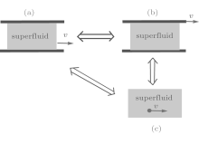
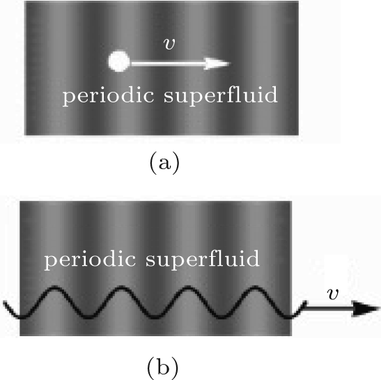
Superfluid is a special kind of fluid which does not suffer dissipation when flowing through a tube. It loses its superfluidity only when its speed exceeds a certain critical value. The superfluidity of liquid helium 4 was first explained by Landau.[10] He considered a superfluid moving inside a stationary tube with velocity v. Since the system is invariant under the Galilean transformation, this scenario is equivalent to a stationary fluid inside a moving tube. If the elementary excitation in a stationary superfluid with momentum q has energy ε 0(q), then the energy of the same excitation in the background of a moving fluid with v is ε v(q) = ε 0(q) + v· q. A fluid experiences friction only through emitting elementary excitations, and it is a superfluid if these elementary excitations are energetically unfavorable. In other words, a superfluid satisfies the constraint ε v(q) > 0. It readily leads to the well-known Landau’ s criterion for superfluid,

Here vc is the critical velocity of the superfluid, which is determined by the smallest slope of the excitation spectrum of a stationary superfluid.
Another way of deriving the formula of critical velocity is from the point view of Cerenkov radiation. Consider a macroscopic impurity moving in the superfluid generates an excitation. According to the conservations of both momentum and energy, we should have


where m0 is the mass of the impurity, vi and vf are the initial and final velocities of the impurity, respectively. The above two conservations (2) and (3) cannot be satisfied simultaneously when

The critical velocity vc here has the same expression as that obtained from Landau’ s criterion. If the excitations are phonons, i.e., ε 0(q) = c| q| , then vc < c. This means that the impurity could not generate phonons in the superfluid and would not experience any viscosity when its speed was smaller than the sound speed. This is in fact nothing but the Cerenkov radiation, [12– 14] where a charged particle radiates only when its speed exceeds the speed of light in the medium. There is also interesting work discussing the possible deviation from this relation.[16]
These two different ways of derivation are equivalent when the system has the Galilean invariance. By transforming to another reference frame illustrated in Fig. 1(b), the superfluid can be viewed as being dragged by a moving tube. We then replace the moving tube with a macroscopic impurity moving inside the superfluid as shown in Fig. 1(c). Consequently, for systems with Galilean invariance, the critical velocity of a superfluid moving inside a tube without experiencing friction is just the critical velocity of an impurity moving in a superfluid without generating excitations. For systems without the Galilean invariance, such an equivalence is lost as we will see later with the spin– orbit coupled BEC.
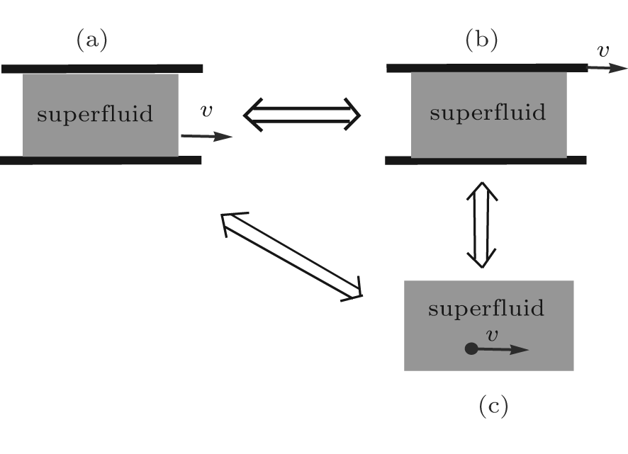 | Fig. 1. (a) A superfluid moves inside a stationary tube. (b) The superfluid is dragged by a tube moving at the speed of v. (c) An impurity moves at v in the superfluid. The two-way arrow indicates the equivalence between different scenarios. |
For ultracold bosonic gases, the low-energy excitation is phonon, linear with respect to momentum q, thus the critical speed of this superfluid is just the sound speed. Taking into account the non-uniformity of the trapped gas, the critical velocity measured in experiments agrees well with the value predicted by Landau’ s theory.[17] For liquid helium 4, as there is another kind of elementary excitations called rotons, the critical speed of superfluid helium 4 is largely determined by the roton excitation, much smaller than its sound speed. Nevertheless, the critical velocity measured in experiments is still one order of magnitude smaller than the value predicted by the theory.[18] Therefore, it is remarkable that Landau’ s prediction of critical velocity was experimentally confirmed with BEC almost six decades after its invention.
One remark is warranted on Landau’ s theory of superfluidity. Landau’ s criterion (1) of critical speed does not apply for many superfluids. However, Landau’ s energetic argument for superfluidity is very general and can be applied to all the cases considered in this review. We shall use this argument to determine the critical speeds of various superfluids.
As liquid helium 4 is a strongly-interacting system, the theoretical calculation of its excitation spectrum is challenging. However, for a dilute ultracold bosonic gases, convenient yet precise approximations can be made to determine its excitation in theory. Due to the dilute nature and short-range interaction, the interaction between atoms can be approximated by a contact interaction. Furthermore, for low energy scattering of bosonic atoms, the s-wave scattering channel dominates. Hence, as a good approximation, the actual complex interaction between atoms is replaced by an effective s-wave contact interaction, i.e., U(r1, r2) = 4π ħ 2aδ (r1 − r2)/M, where a is the s-wave scattering length. At zero temperature, assume all the particles condense into the same orbit ψ (r), then its evolution is governed by the mean field Gross– Pitaevskii (GP) equation, [19]

where V(r) is the trapping potential or other external potential, and c = 4π ħ 2a/M is the interaction parameter or coupling constant. The GP energy functional reads
Note that here the wave function ψ is normalized to the total particle number N. The approximation we make here is the mean-field approximation, and the interaction between atoms is replaced by an effective mean-field potential. The validity of the approximation usually depends on the condensed fraction. For weakly interacting dilute bosonic gases near zero temperature, the condensed fraction can be more than 90 percent. In these situations, the GP equation works well. It has been used to calculate the collective excitations of trapped BEC, as well as vortex dynamics. Pretty good agreement is achieved between theory and experiment. With a stochastic term describing the effect of thermal atoms, the modified stochastic GP equation can also simulate BEC systems at finite temperature.[20, 21] In addition, for atoms with spin, one can also derive a multi-component GP equation to describe a spinor superfluid.[22]
The stationary state the GP equation describes is a zeroth-order approximation in some sense. It only takes into account the interaction between the condensed particles. The first-order approximation is to take into account the interaction between the condensed particles and un-condensed particles. This is settled by the Bogoliubov theory of elementary excitations.[23] The standard Bogoliubov theory is to diagonalize the mean-field Hamiltonian by the Bogoliubov transformation. Here we adopt an equivalent yet more convenient way to deal with this problem in inhomogeneous systems. For a stationary state ψ (r, t) that satisfies the GP equation, we consider some small time-dependent perturbations δ ψ (r, t) added to this stationary state. The perturbed state Ψ = ψ + δ ψ also satisfies the GP equation,

Expanding this equation to first order in the perturbation δ ψ , one arrives at the equation of motion of the perturbation δ ψ (r, t),

and its complex conjugate partner. Assume the state before perturbation is a stationary state with the wave function 


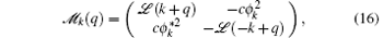
where the matrix 𝓜 is given by

with H0 = − ħ 2∇ 2/2M + V(r) − μ + 2cn(r). By diagonalizing 𝓜 , one obtains two sets of solutions, but only the solution satisfying the constraint 

As a specific example, we apply the above formalism to the uniform Bose gas, namely, putting V(r) = 0. The wave function before perturbation is just 


where 

The method of mean-field approximation and Bogoliubov transformation is very general, and applies in other more complicated situations. In the following discussion, we use this method to study three types of superfluids, superfluid in a periodic potential, superfluid with spin– orbit coupling and superfluid of pure spin current.
It is hard to change the density of helium 4 as it is a liquid. In contrast, we can easily modulate the density of a BEC which is a gas. When we put a BEC in an optical lattice, we obtain a superfluid whose density is periodically modulated. One can even further periodically modulate the interatomic interaction of the BEC with optical Feshbach resonance.[25] Supersolid helium 4 may be also regarded as a periodic superfluid as it can be viewed as some superfluid defects (most likely vacancies) flowing in a helium solid lattice.[26, 27] In this section, we use a BEC in an optical lattice as an example to examine the properties of a periodic superfluid. Compared to the uniform superfluid in free space, a new type of instability, i.e., the dynamical instability is found when the quasi-momentum k of the superfluid is larger than a critical value. Usually the dynamical instability dominates the accompanying Landau instability as it happens on a much faster time scale.[28] The presence of the periodic potential also brings along another critical velocity.
Now we study the superfluidity of a BEC in a periodic potential, [29, 30] which is provided by the optical lattice in cold atom experiments. For simplicity, we consider a quasi-one-dimensional BEC, confined in a cigar-shaped trap. We treat the system with the mean-field theory and obtain the grand-canonical GP Hamiltonian as

where all the variables are scaled to be dimensionless with respect to a set of characteristic parameters of the system, the atomic mass M, the wave number kL of the laser light generating the optical lattice, and the average density n0 of the BEC. The chemical potential μ and the strength of the periodic potential v are in units of 


For non-interacting case (c = 0), diagonalizing the Hamiltonian will give the standard Bloch waves and energy bands. When the mean-field interaction is turned on (c ≠ 0), in principle the Hamiltonian allows for other types of solutions which have no counterpart in the non-interacting case.[31, 32] Here we focus on the solutions which still have the form of Bloch waves, i.e., ψ k(x) = eikxϕ k(x), where ϕ k(x) has the same period with the optical lattice. ϕ k(x) can be found by extremizing the Hamiltonian above.[30] The solution found in this way should satisfy the stationary GP equation with periodic potential,

To determine the superfluidity of these Bloch states, we must consider elementary excitations around these Bloch states, and check whether the excitation energy is always positive. Positive excitation energy indicates that the Bloch state is a local energy minimum, and it is stable against small perturbations. Due to the periodicity of the Bloch wave, the perturbations can be decomposed into different decoupled modes labeled by q,

where q ranges between − 1/2 and 1/2, and the perturbation functions uk and vk are of periodicity of 2π .
Following the similar method in Section 2.2, we linearize the GP equation above to obtain the Bogoliubov equation that uk and vk satisfy

where
with
This eigenvalue equation has two sets of solutions, with one corresponding to physical excitations, which is mostly phonon excitation, and the other called anti-phonon that is not physical. If the physical excitation ε k(q) is positive, the Bloch wave ψ k is a local minimum, and the system will have superfluidity. Otherwise, the system suffers Landau instability or dynamical instability, depending on whether ε k(q) is real negative or complex.
In the case of free space v = 0, the Bloch state ψ k becomes a plane wave eikx. Then the operator 𝓜 k(q) becomes

and we recover the excitations in the uniform case

We immediately see that the excitation energy is always real, which means that the BEC flows in free space are always dynamically stable.
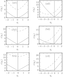
When there is a periodic potential, the situation is dramatically different, where the excitation energy can have imaginary part, signaling the dynamical instability of the system. By numerically solving the Bogoliubov equation above, we show the stability phase diagrams for BEC Bloch waves in the panels of Fig. 2, where different values of v and c are considered. The results have reflection symmetry in k and q, so we only show the parameter region, 0 ≤ k ≤ 1/2 and 0 ≤ q ≤ 1/2. In the shaded area (light or dark) of each panel of Fig. 2, the excitation energy is negative, and the corresponding Bloch states ψ k are saddle points. For those values of k outside the shaded area, the Bloch states are local energy minima and represent superfluids. The superfluid region expands with increasing atomic interaction c, and occupies the entire Brillouin zone for sufficiently large c. On the other hand, the lattice potential strength v does not affect the superfluid region very much as we see in each row. The phase boundaries for v ≪ 1 are well reproduced from the analytical expression 
 | Fig. 2. Stability phase diagrams of BEC Bloch states in optical lattices. k is the wave number of BEC Bloch waves; q denotes the wave number of perturbation modes. In the shaded (light or dark) area, the perturbation mode has negative excitation energy; in the dark shaded area, the mode grows or decays exponentially in time. The triangles in (a1– a4) represent the boundary, q2/4 + c = k2, of saddle point regions at v = 0. The solid dots in the first column are from the analytical results of Eq. (20). The circles in (b1) and (c1) are based on the analytical expression (21). The dashed lines indicate the most unstable modes for each Bloch wave ψ k.[29] |
If ε k(q) is complex, the system suffers dynamical instability, which is shown by the dark-shaded areas in Fig. 2. The dynamical instability is the result of the resonance coupling between a phonon mode and an anti-phonon mode by first-order Bragg scattering. The matrix 𝓜 k(q) is real in the momentum representation, meaning that its complex eigenvalue can appear only in conjugate pairs and they must come from a pair of real eigenvalues that are degenerate prior to the coupling. Degeneracies or resonances within the phonon spectrum or within the anti-phonon spectrum do not give rise to dynamical instability; they only generate gaps in the spectra. Based on this general conclusion, we consider two special cases, which allow for simple explanations of the onset of dynamical instability.
One case is the weak periodic potential limit v ≪ 1, where we can approximate the boundary with the free space case. This case corresponds to the first column of Fig. 2. In this limit, we can approximate the phonon spectrum and the anti-phonon spectrum with the ones given by Eq. (19). By equating them, ε + (q − 1) = ε − (q). For the degeneracy, we find that the dynamical instability should occur on the following curves:

These curves are plotted as solid dots in Fig. 2, and they fall right in the middle of the thin dark-shaded areas. To some extent, one can regard these thin dark-shaded areas as broadening of the curves (20). It is noted in Ref. [33] that the relation (20) is also the result of ε + (q − 1) + ε + (− q) = 0, which involves only the physical phonons. Therefore, the physical meaning of Eq. (20) is that one can excite a pair of phonons with zero total energy and with total momentum equal to a reciprocal wave number of the lattice.
The other case, c ≪ v, is shown in the first row of Fig. 2. The open circles along the left edges of these dark-shaded areas are given by

where E1(k) is the lowest Bloch band of

In this linear periodic system, the excitation spectrum (phonon or anti-phonon) just corresponds to transitions from the Bloch states of energy E1(k) to other Bloch states of energy En(k + q), or vise versa. The above equation is just the resonance condition between such excitations in the lowest band (n = 1). Alternatively, we can write the resonance condition as

Thus, this condition may be viewed as the energy and momentum conservation for two particles interacting and decaying into two different Bloch states E1(k + q) and E1(k − q). This is the same physical picture behind Eq. (20).
One common feature of all the diagrams in Fig. 2 is that there are two critical Bloch wave numbers, kt and kd. Beyond kt the Bloch waves ψ k suffer the Landau instability; beyond kd the Bloch waves ψ k are dynamically unstable. The onset of instability at kd always corresponds to q = 1/2. In other words, if we drive the Bloch state ψ k from k = 0 to k = 1/2 the first unstable mode is always q = ± 1/2, which represents period doubling. Only for k > kd can longer wavelength instabilities occur. The growth of these unstable modes drives the system far away from the Bloch state and spontaneously breaks the translational symmetry of the system.
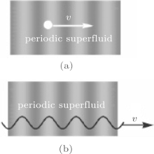
Besides inducing the dynamical instability, the presence of the optical lattice has also non-trivial consequences on the concept of critical velocity. In contrast to the homogeneous superfluid which has only one critical velocity, there are two distinct critical velocities for a periodic superfluid.[34] The first one, which we call inside critical velocity, is for an impurity to move frictionlessly in the periodic superfluid system (Fig. 3(a)); the second, which is called trawler critical velocity, is the largest velocity of the lattice for the superfluidity to maintain (Fig. 3(b)). We illustrate these two critical velocities with a BEC in a one-dimensional optical lattice.
 | Fig. 3. (a) A macroscopic obstacle moves with a velocity of v inside a superfluid residing in a periodic potential. The superfluid and periodic potential are “ locked” together and there is no relative motion between them. (b) The lattice where a superfluid resides is slowly accelerated to a velocity of v. |
The presence of the optical lattice plays a decisive role in the appearance of the two critical velocities: two very different situations can arise. The first situation is described in Fig. 3(a), where one macroscopic impurity moves inside the superfluid. The key feature in this situation is that there is no relative motion between the superfluid and the lattice. The other situation is illustrated in Fig. 3(b), where the lattice is slowly accelerated to a given velocity and there is a relative motion between the superfluid and the lattice. For these two different situations, two critical velocities naturally arise.
In the first scenario, we consider a moving impurity that generates an excitation with momentum q and energy ε 0(q) in the BEC. According to the conservations of both momentum and energy, we should have


where m0 is the mass of the impurity, vi and vf are the initial and final velocities of the impurity, respectively, G is the reciprocal vector, and ε 0(q) is the excitation of the BEC at the lowest Bloch state k = 0. Note that in contrast to the conservation of momentum in free space, here the total momentum of the impurity and the excitation is not exactly conserved due to the presence of an optical lattice, and the momenta differing by integer multiples of reciprocal lattice vector are equivalent. For phonon excitations, i.e., ε 0(q) = c| q| , these two conservations can always be satisfied simultaneously no matter how small the velocity of the impurity is. In other words, the critical velocity for this scenario is exactly zero.
In the other scenario, there is relative motion between the superfluid and the optical lattice, and the superfluid no longer resides in the k = 0 point of the Brillouin zone. We should examine the stability of Bloch waves with nonzero k, which is discussed in detail in the previous subsection. The critical wave number kt mentioned above corresponds precisely to the trawler critical velocity vt here. As kt is not zero, vt is not zero.
Both critical velocities can be measured with BECs in optical lattices. The inside critical velocity vi can be measured with the same experimental setting as that in Ref. [35], where the superfluidity of a BEC was studied by moving a blue-detuned laser inside the BEC. For the trawler critical velocity vt, one can repeat the experiment in Ref. [28], where a BEC is loaded in a moving optical lattice. One only needs to shift his attention from dynamical instability to superfluidity. The potential difficulty lies in that the Landau instability occurs over a much larger time scale, which may be beyond the life time of a BEC.[28]
The intrinsic spin– orbit coupling (SOC) of electrons plays a crucial role in many exotic materials, such as topological insulators.[36, 37] In spintronics, [38] its presence enables us to manipulate the spin of electrons by means of exerting electric field instead of magnetic field, which is much easier to implement for industrial applications. However, as a relativistic effect, the intrinsic SOC does not exist or is very weak for bosons in nature. With the method of engineering atom– laser interaction, an artificial SOC has been realized for ultracold bosonic gases in Refs. [39]– [42]. A great deal of effort has been devoted to study many interesting properties of spin– orbit coupled BECs.[43– 55]
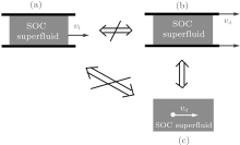
A dramatic change that the SOC brings to the concept of superfluidity is the breakdown of Landau’ s criterion of critical velocity (1) and the appearance of two different critical velocities. Laudau’ s criterion of the critical velocity (1) is based on the Galilean invariance. It is apparent to many that the scenario where a superfluid flows inside a motionless tube is equivalent to the other scenario where a superfluid at rest is dragged by a moving tube. If the flowing superfluid loses its superfluidity when its speed exceeds a critical speed vc, then the superfluid in the other scenario will be dragged into motion by a tube moving faster than vc. However, this equivalence is based on that the superfluid is invariant under the Galilean transformation. As SOC breaks the Galilean invariance of the system, [56] we find that the two scenarios mentioned above are no longer equivalent as shown in Fig. 4: the critical speed for scenario (a) is different from the one for scenario (b). For easy reference, the critical speed for (a) is hereafter called the critical flowing speed and the one for (b) the critical dragging speed.
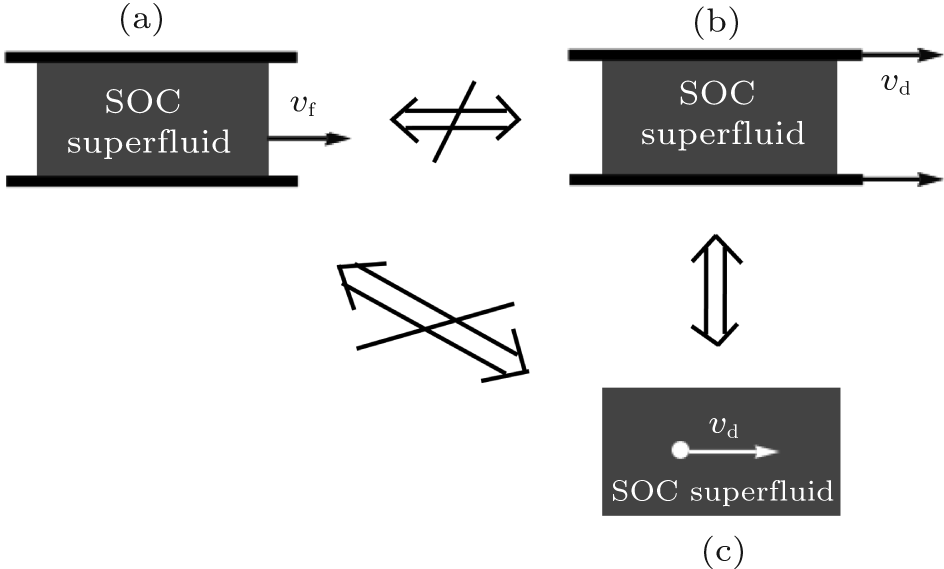 | Fig. 4. (a) A superfluid with SOC moves while the tube is at rest. (b) The superfluid is dragged by a tube moving at the speed of v. (c) An impurity moves at v in the SOC superfluid. The reference frame is the lab. The two-way arrow indicates the equivalence between different scenarios and the arrow with a bar indicates the non-equivalence. |
For ultra-cold atomic gases, the breakdown of the Galilean invariance in the presence of SOC can be understood both theoretically and experimentally.
From the theoretical point of view, we show in detail how a system with SOC changes under the Galilean transformation. We adopt the formalism in Ref. [56]. The operator for the Galilean transformation is

which satisfies the definition


A system is invariant under the Galilean transformation if the following equation is satisfied (Ref. [56]):

The above condition is clearly satisfied by a Hamiltonian without SOC, e.g., H = p2/2m. However, for a Hamiltonian with SOC, e.g., Hsoc = p2/2m + γ (σ xpy − σ ypx), it is easy to check that

where 
In the experiments of ultra-cold atomic gases, the SOC is created by two Raman beams that couple two hyperfine states of the atom. Since the Galilean transformation only boosts the BEC, not including the laser setup as a whole, the moving BEC will experience a different laser field due to the Doppler effect, resulting in a loss of the Galilean invariance.
We use the method introduced in Section 2.2 to study the superfluidity of a BEC with SOC by computing its elementary excitations.[57] In experiments, only the equal combination of Rashba and Dresselhaus coupling is realized. Here we use the Rashba coupling as an example as the main conclusion does not rely on the details of the SOC type.
We calculate how the elementary excitations change with the flow speed and manage to derive from these excitations, the critical speeds for the two different scenarios shown in Fig. 4(a) and 4(b). We find that there are two branches of elementary excitations for a BEC with SOC: the lower branch is phonon-like at long wavelengths and the upper branch is generally gapped. Careful analysis of these excitations indicates that the critical flowing velocity for a BEC with SOC (Fig. 4(a)) is non-zero, while the critical dragging speed is zero (Fig. 4(b)). This shows that the critical velocity depends on the reference frame for a BEC with SOC and, probably, for any superfluid that has no Galilean invariance.
Specifically, we consider a BEC with pesudospin 1/2 and the Rashba SOC. The system can be described by the Hamiltonian[44, 47, 58, 59]

where γ is the SOC constant, C1 and C2 are interaction strengths between the same and different pesudospin states, respectively. For simplicity and easy comparison with previous theory, we focus on the homogeneous case V(r) = 0 despite that the BEC usually resides in a harmonic trap in experiments. Besides, we limit ourselves to the case C1 > C2, namely, in the plane wave phase. In the following discussion, for simplicity, we set ħ = M = 1 and ignore the non-essential z direction, treating the system as two-dimensional. We also assume the BEC moves in the y direction, and the critical velocity is found to be not influenced by the excitation in the z direction.
The GP equation obtained from the Hamiltonian (32) has plane wave solutions
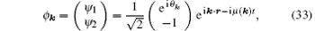
where tanθ k = kx/ky and μ (k) = | k| 2/2 − γ | k| + (C1 + C2)/2. The solution ϕ k is the ground state of the system when | k| = γ . There are another set of plane wave solutions, which have higher energies and are not relevant to our discussion.
We study first the scenario depicted in Fig. 4(a), where the BEC flows with a given velocity. Since the system is not invariant under the Galilean transformation, we cannot use Laudau’ s argument to find the excitations for the flowing BEC from the excitation of a stationary BEC. We have to compute the excitations directly. This can be done by computing the elementary excitations of the state ϕ k with the Bogoliubov equation for different values of k.
Without loss of generality, we choose k = kŷ with k > 0. Following the standard procedure of linearizing the GP equation, [29, 30] we have the following Bogoliubov equation:

where
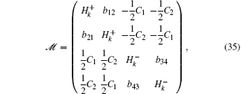
with

and

As usual, there are two groups of eigenvalues and only the ones whose corresponding eigenvectors satisfy | ui| 2 − | vi| 2 = 1 (i = 1, 2) are physical.
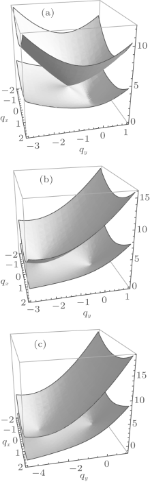
In general there are no simple analytical results. We have numerically diagonalized 𝓜 to obtain the elementary excitations. We find that part of the excitations are imaginary for BEC flows with | k| < γ . This means that all the flows with | k| < γ are dynamically unstable and therefore do not have superfluidity. For other flows with k ≥ γ , the excitations are always real and they are plotted in Fig. 5. One immediately notices that the excitations have two branches, which contact each other at a single point. Closer examination shows that the upper branch is gapped in most of the cases, while the lower branch has phonon-like spectrum at large wavelengths. These features are more apparent in Fig. 6, where only the excitations along the x axis and y axis are plotted.
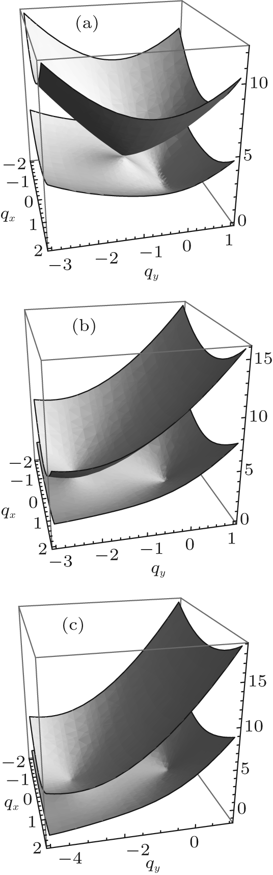 | Fig. 5. Elementary excitations of a BEC flow with the SOC. (a) k = 1; (b) k = 3; (c) k = 4. C1 = 10, C2 = 4, and γ = 1. |
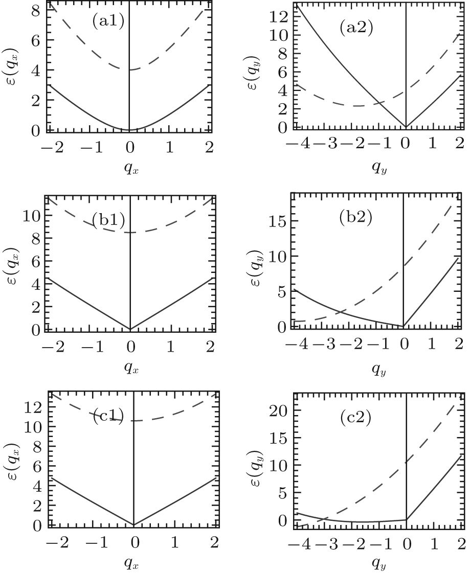 | Fig. 6. Excitations along the x axis (the first column) and y axis (the second column) at different values of k. (a1, a2) k = 1; (b1, b2) k = 3; (c1, c2) k = 4. C1 = 10, C2 = 4, and γ = 1. |
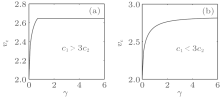
In Figs. 5(c) and 6(c2), we note that part of the excitations in the upper branch are negative, indicating that the underlying BEC flow is thermodynamically unstable and has no superfluidity. In fact, our numerical computation shows that there exists a critical value kc: when k > kc either part of the upper branch of excitations or part of the lower branch or both become negative. This means that the flows described by the plane wave solution ϕ k, − with | k| > kc suffer Landau instability and have no superfluidity. Together with the fact that the flows with | k| < γ are dynamically unstable, we can conclude that only the flows with γ ≤ | k| ≤ kc have superfluidity. The corresponding critical speed is vc = kc − γ . We have plotted how the critical flowing velocity vc varies with the SOC parameter γ (Fig. 7).
 | Fig. 7. Critical flowing velocity vc of a BEC as a function of the SOC parameter γ . (a) C1 = 11, C2 = 3; (b) C1 = 14, C2 = 6. |
We turn to another reference frame illustrated in Fig. 4(b), where the BEC can be viewed as being dragged by a moving tube. To simplify the discussion, we replace the moving tube with a macroscopic impurity moving inside the BEC as shown in Fig. 4(c). Correspondingly, the question “ whether the BEC will be dragged along by the moving tube?” is replaced by an equivalent question “ whether the impurity will experience any viscosity?” . Suppose that the moving impurity generates an excitation in the BEC. According to the conservations of both momentum and energy, we should have


as those for a BEC without SOC, where ε 0(q) is the excitation of the BEC at k = γ . The critical dragging velocity derived from Eqs. (36) and (37) is given by
If the excitations were pure phonons, i.e., ε 0(q) = c| q| , these two conservations would not be satisfied simultaneously when v ≈ | vi| ≈ | vf| < c. This means that the impurity could not generate phonons in the superfluid and would not experience any viscosity when its speed was smaller than the sound speed. Unfortunately, for our BEC system, the elementary excitations ε 0(q) are not pure phonons, as will be shown below.
When γ ≠ 0, the excitations ε 0(q) also share two branches. Along the x axis, these two branches are

where s1 = 2γ 4 + γ 2(C1 − C2), 


When γ > 0, the upper branch 

This shows that 
We have also investigated the superfluidity with the general form of SOC, which is a mixture of Rashba and Dresselhaus coupling. Mathematically, this SOC term has the form α σ xpy − β σ ypx. The essential physics is the same: the critical flowing speed is different from the critical dragging speed, and therefore the critical velocity depends on the choice of the reference frame. However, the details do differ when α ≠ β . The critical dragging speed is no longer zero. Without loss of generality, we let α > β . The slope of the excitation spectrum for the ground state along the y axis is

and the slope along the x axis,

The critical dragging velocity is the smaller one of the above two slopes, both of which are nonzero.
Spin– orbit coupled BECs have been realized by many different groups[39– 42] through coupling ultracold 87Rb atoms with laser fields. The strength of the SOC in the experiments can be tuned by changing the directions of the lasers[39– 41] or through the fast modulation of the laser intensities.[60] The interaction between atoms can be adjusted by varying the confinement potential, the atom number or through the Feshbach resonance.[6] For the scenario in Fig. 4(b), one can use a blue-detuned laser to mimic the impurity for the measurement of the critical dragging speed similar to the experiment in Ref. [61]. For the scenario in Fig. 4(a), there are two possible experimental setups for measuring the critical flowing speed. In the first one, one generates a dipole oscillation similar to the experiment in Ref. [41] but with a blue-detuned laser inserted in the middle of the trap. The second one is more complicated. At first, one can generate a moving BEC with a gravitomagnetic trap.[62] One then uses Bragg spectroscopy[63, 64] to measure the excitations of the moving BEC, from which the superfluidity can be inferred. For the typical atomic density of 1014– 1015 cm− 3 achievable in current experiments, [61] and the experimental setup in Ref. [39], the critical flowing velocity is 0.2– 0.6 mm/s, while the critical dragging velocity is still very small, about 10− 3– 10− 2 mm/s. To further magnify the difference between the two critical velocities, one may use the Feshbach resonance to tune the s-wave scattering length.
A neutral boson can carry both mass and spin; it thus can carry both mass current and spin current. However, when a boson system is said to be a superfluid, it traditionally refers only to its mass current. The historical reason is that the first superfluid discovered in experiment is the spinless helium 4 which carries only mass current. For a boson with spin, say, a spin-1 boson, we can in fact have a pure spin current, a spin current with no mass current. This pure spin current can be generated by putting an unpolarized spin-1 boson system in a magnetic field with a small gradient. Can such a pure spin current be a superflow? In this section we try to address this issue for both planar and circular pure spin currents by focusing on an unpolarized spin-1 Bose gas.
The stability of a pure spin current in an unpolarized spin-1 Bose gas was studied in Ref. [65]. It was found that such a current is generally unstable and is not a superflow. We have recently found that the pure spin current can be stabilized to become a superflow:[66] (i) for a planar flow, it can be stabilized with the quadratic Zeeman effect; (ii) for a circular flow, it can be stabilized with SOC. We shall discuss these results and related experimental schemes in detail in the next subsections.
There has been lots of studies on the counterflow in a two-species BEC, [65, 67– 77] which appears very similar to the pure spin current discussed here. It was found that there is a critical relative speed beyond which the counterflow state loses its superfluidity and becomes unstable.[67– 75] We emphasize that the counterflow in a two-species BEC is not a pure spin current for two reasons. Firstly, although pesudospin the two species may be regarded as two components of a pesudospin 1/2, they do not have SU(2) rotational symmetry. Secondly, it is hard to prepare experimentally a BEC with exactly equal numbers of bosons in the two species to create a counterflow with no mass current. There is also interesting work addressing the issue of spin superfluidity in other situations.[78– 81]
We consider a spin-1 BEC in free space. The mean-field wave function of such a spin-1 BEC satisfies the following GP equation:[82]

where ψ m (m = 1, 0, − 1) are the components of the macroscopic wave function, 
We consider a spin current state of the above GP equation with the form
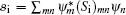
where n is the density of the uniform BEC. The wave function above describes a state with component m = 1 moving at speed ħ k1/M, component m = − 1 moving at speed ħ k2/M, and component m = 0 stationary. The requirement of equal chemical potential leads to | k1| = | k2| . In the case where k1 = − k2, this state carries a pure spin current: the total mass current is zero as it has equal mass counterflow while the spin current is nonzero.
To determine whether the state (46) represents a superfluid, we need to compute its Bogoliubov excitation spectrum, also using the method introduced in Section 2.2. It is instructive to first consider the special case where there is no counterflow, i.e., k1 = k2 = 0. The excitation spectra are found to be 


For the counterflow state with k1 = − k2 ≠ 0, the stability has been studied in Ref. [65]. It is found that, for the antiferromagnetic interaction case (c0 > 0, c2 > 0), the excitation spectrum of the m = 0 component always has nonzero imaginary part in the long-wavelength limit as long as there is counterflow between the two components, and the imaginary excitations in the m = 1, − 1 components only appear for a large enough relative velocity 
For the general non-collinear case (k = (k1 + k2)/2 ≠ 0) and antiferromagnetic interaction, the excitation spectrum for the m = 0 component is found to be
We see here that as long as the momenta of the two components are not exactly parallel, i.e., k1 is not exactly equal to k2, then | k| < | k1| , and there is always dynamical instability for the long-wavelength excitations.
Therefore, the spin current in Eq. (46) is generally unstable and not a superflow. This instability originates from the interaction process described by 
The above intuitive argument can be made more rigorous and quantitative. Consider the case k1 = − k2. With the quadratic Zeeman term, the excitation spectrum for the m = 0 component changes to

Therefore, as long as − λ − ħ 2| k1| 2/2M > 0, long-wavelength excitations will be stable for the m = 0 component. From the excitation of the m = 0 component, one can obtain a critical relative velocity of the spin current, 

In the cylindrical geometry, we consider a pure spin current formed by two vortices with opposite circulation in the m = 1, − 1 components. From similar arguments, one can expect that interaction will make such a current unstable. Inspired by the quadratic Zeeman effect method above, we propose to use SOC to stabilize it. The SOC can be viewed as a momentum-dependent effective magnetic field that is exerted only on the m = 1, − 1 components. Therefore, it is possible that SOC lowers the energy of m = 1, − 1 components and, consequently, suppresses the interaction process leading to the instability.
The model of a spin-1 BEC subjecting to the Rashba SOC can be described by the following energy functional:
where ρ is the density, V(r) = Mω 2(x2 + y2)/2 is the trapping potential, and γ is the strength of SOC. 〈 · · · 〉 is the expectation value taken with respect to the three component wave function ψ = (ψ 1, ψ 0, ψ − 1)T. Here we assume the confinement in the z direction is very tight with trapping frequency ħ ω z ≫ μ , kBT, μ being the chemical potential and T the temperature, and have integrated the model with respect to the z direction to obtain an effective two-dimensional system. The two-dimensional coupling constants are related to the three-dimensional scattering lengths through the relations, 


The above model can describe a spin-1 BEC of 23Na confined in a pancake harmonic trap. Assume the atom number is about 105. Using the estimate of scattering lengths a0 = 50aB, a2 = 55aB, [84] with aB being the Bohr radius, the ground state of spin-1 23Na should be antiferromagnetic because c̃ 0 > 0 and c̃ 2 > 0.[45] Previous studies of spin-1 BEC with Rashba SOC mostly focus on the strong SOC regime, where the ground state is found to be the plane-wave phase or the stripe phase, for ferromagnetic interaction and antiferromagnetic interaction, respectively.[44] Here we are interested in the antiferromagnetic interaction case and the weak SOC regime (κ ≪ 1), and calculate the ground-state wave function of the energy functional with the method of imaginary time evolution.
We find that when the SOC is weak (κ ≪ 1), the ground-state wave function has the form

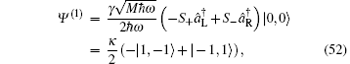
with χ 1(r) = − χ − 1(r) and all χ i real. The ground state is shown in Fig. 8. Such a ground state consists of an anti-vortex in the m = 1 component and a vortex in the m = − 1 component. The m = 0 component does not carry angular momentum. Since | ψ 1| = | ψ − 1| , the net mass current vanishes.
 | Fig. 8. Amplitudes (a1, b1, c1) and phase angles (a2, b2, c2) of the three component wave function ψ = (ψ 1, ψ 0, ψ − 1)T at the ground state of Hamiltonian (49) for a BEC of 23Na confined in a pancake trap. The particle number is 105, the radial frequency of the trap is 2π × 55 Hz, and the dimensionless SOC strength is κ = 0.04. The confinement in the z direction is very tight with ω z = 2π × 4200 Hz, so the system is effectively two-dimensional. Units of the X and Y axes are ah. |
The wave function (50) can be understood at the single-particle level. In terms of the ladder operators of spin and angular momentum, the SOC term reads

where S± is the ladder operator of spin, and 
where | ms, mo〉 denotes a state with spin quantum number ms and orbital magnetic quantum number mo. One immediately sees that ψ 1 has angular momentum − ħ and ψ − 1 has angular momentum ħ . In addition, the amplitudes of both ψ 1 and ψ − 1 are proportional to κ .
There exits a continuity equation for the spin density and spin current, which is

The spin current density tensor 
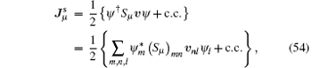
where

and c.c. means the complex conjugate. The second part in vnl is induced by the SOC.
By the definition in Eq. (54), the spin current density carried by the ground state (50) is
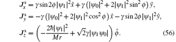
From both analytical and numerical results of the wave function, | ψ 1| ≪ | ψ 0| , so 


 | Fig. 9. Distribution of the spin current densities    |
In this subsection, we propose the experimental schemes to generate and detect the pure spin currents discussed in Subsections 5.1 and 5.2.
The planar pure spin current can be easily generated. By applying a magnetic field gradient, the two components m = 1, − 1 will be accelerated in opposite directions and a pure spin current is generated as done in Refs. [70] and [71]. To stabilize this spin current, one needs to generate the quadratic Zeeman effect. We apply an oscillating magnetic field Bsinω t with the frequency ω being much larger than the characteristic frequency of the condensate, e.g., the chemical potential μ . The time averaging removes the linear Zeeman effect; only the quadratic Zeeman effect remains. The coefficient of the quadratic Zeeman effect from the second-order perturbation theory is given by λ = (gμ BB)2/Δ Ehf, where g is the Landé g factor of the atom, μ B is the Bohr magneton, and Δ Ehf is the hyperfine energy splitting.[88] For the F = 2 manifold of 87Rb, Δ Ehf < 0, so the coefficient of the quadratic Zeeman effect is negative.
The circular flow in Subsection 5.2 may find prospective realizations in two different systems: cold atoms and exciton BEC. In cold atoms, we consider a system consisting of a BEC of 23Na confined in a pancake trap, where the confinement in the z direction is so tight that one can treat the system effectively as two-dimensional. The SOC can be induced by two different methods. One is by the exertion of a strong external electric field E in the z direction. Due to the relativistic effect, the magnetic moment of the atom will experience a weak SOC, where the strength γ = gμ B| E| /Mc2. Here M is the atomic mass and c is the speed of light. For weak SOC (small γ ), the fraction of atoms in the m = 1, − 1 components is proportional to γ 2. For an experimentally observable fraction of atoms, e.g., 0.1% of 105 atoms, using the typical parameters of 23Na BEC, the estimated electric field is of the same order of magnitude as the vacuum breakdown field. For atoms with smaller mass or larger magnetic moment, the required electric field can be lowered. Another method of realizing SOC is to exploit the atom laser interaction, where strong SOC can be created in principle.[89] In exciton BEC systems, as the effective mass of exciton is much smaller than that of atom, the required electric field is four to five orders of magnitude smaller, which is quite feasible in experiments.[90– 93]
The vortex and anti-vortex in the m = 1, − 1 components can be detected by the method of time of flight. First one can split the three spin components with the Stern– Gerlach effect. The appearance of vortex or anti-vortex in the m = 1, − 1 components is signaled by a ring structure in the time-of-flight image. After a sufficiently long expansion time, the ring structure should be clearly visible.
In summary, we have studied the superfluidity of three kinds of unconventional superfluids, which show distinct features from a uniform spinless superfluid. The periodic superfluid may suffer a new type of instability, the dynamical instability, absent in homogeneous case; the spin– orbit coupled superfluid has a critical velocity dependent on the reference frame, a new phenomenon compared with all previous Galilean invariant superfluids; the superfluid of a pure spin current, though scarcely stable in previous studies, can be stabilized by the quadratic Zeeman effect and SOC in planar and circular geometry, respectively. These new superfluids significantly enrich the physics of bosonic superfluids.
With the rapid advances in cold atom physics and other fields, the family of superfluids is expanding with the addition of more and more novel superfluids. Previous study has greatly deepened and enriched our understanding of superfluidity, but we believe more exciting physics beyond the scope of our current understanding remains to be discovered in the future.
| 1 |
|
| 2 |
|
| 3 |
|
| 4 |
|
| 5 |
|
| 6 |
|
| 7 |
|
| 8 |
|
| 9 |
|
| 10 |
|
| 11 |
|
| 12 |
|
| 13 |
|
| 14 |
|
| 15 |
|
| 16 |
|
| 17 |
|
| 18 |
|
| 19 |
|
| 20 |
|
| 21 |
|
| 22 |
|
| 23 |
|
| 24 |
|
| 25 |
|
| 26 |
|
| 27 |
|
| 28 |
|
| 29 |
|
| 30 |
|
| 31 |
|
| 32 |
|
| 33 |
|
| 34 |
|
| 35 |
|
| 36 |
|
| 37 |
|
| 38 |
|
| 39 |
|
| 40 |
|
| 41 |
|
| 42 |
|
| 43 |
|
| 44 |
|
| 45 |
|
| 46 |
|
| 47 |
|
| 48 |
|
| 49 |
|
| 50 |
|
| 51 |
|
| 52 |
|
| 53 |
|
| 54 |
|
| 55 |
|
| 56 |
|
| 57 |
|
| 58 |
|
| 59 |
|
| 60 |
|
| 61 |
|
| 62 |
|
| 63 |
|
| 64 |
|
| 65 |
|
| 66 |
|
| 67 |
|
| 68 |
|
| 69 |
|
| 70 |
|
| 71 |
|
| 72 |
|
| 73 |
|
| 74 |
|
| 75 |
|
| 76 |
|
| 77 |
|
| 78 |
|
| 79 |
|
| 80 |
|
| 81 |
|
| 82 |
|
| 83 |
|
| 84 |
|
| 85 |
|
| 86 |
|
| 87 |
|
| 88 |
|
| 89 |
|
| 90 |
|
| 91 |
|
| 92 |
|
| 93 |
|