
Cascading failure in the wireless sensor scale-free networks*
[Liu Hao-Rana), b)†  , Dong Ming-Ru
c) , Yin Rong-Ronga), b) , Han Lia) ]
, Dong Ming-Ru|
|


†Corresponding author. E-mail: liuhaoran@ysu.edu.cn, liu.haoran@ysu.edu.cn
*Project supported by the Natural Science Foundation of Hebei Province, China (Grant No. F2014203239), the Autonomous Research Fund of Young Teacher in Yanshan University (Grant No. 14LGB017) and Yanshan University Doctoral Foundation, China (Grant No. B867).
In the practical wireless sensor networks (WSNs), the cascading failure caused by a failure node has serious impact on the network performance. In this paper, we deeply research the cascading failure of scale-free topology in WSNs. Firstly, a cascading failure model for scale-free topology in WSNs is studied. Through analyzing the influence of the node load on cascading failure, the critical load triggering large-scale cascading failure is obtained. Then based on the critical load, a control method for cascading failure is presented. In addition, the simulation experiments are performed to validate the effectiveness of the control method. The results show that the control method can effectively prevent cascading failure.
Wireless sensor networks (WSNs) are usually deployed in remote and dangerous environment.[1, 2] Nodes in the network are often vulnerable to attacks, natural hazards, and resource depletion.[3– 5] Therefore, much attention has been paid to the research on fault tolerance in WSNs. Previous studies on the fault tolerance in WSNs are almost stationary (static fault tolerance).[6– 9] They can tolerate failure nodes but the effect of failure node on the other nodes is not considered. However, the WSNs node has load and the load changes constantly. When a node fails, its load is redistributed the other nodes of the network. Some of the increased load may then exceed the capacity of their respective node, leading to further failure and eventually to a cascading breakdown of the entire network. This change process of the topology load is called cascading failure.[10] The cascading failure can seriously affect the network performance and even causes network failure. Therefore, in order to ensure the normal operation of the network under nodes failure, it is required that the network topology not only has well static fault tolerance but also can control cascading failure effectively in the process of network operation.
In recent years, studies have found that the scale-free topology with power law distribution has strong fault tolerance to random failure.[11, 12] Then the scale-free structure is introduced into the WSNs and the fault tolerance in WSNs is improved effectively.[13] The scale-free topology structure has strong static fault tolerance but ignoring the cascading failure. Thus, it is significant to research the cascading failure of the scale-free fault tolerant topology in WSNs and then prevent it.
Cascading failure of the scale-free topology has been widely investigated. Motter et al. proposed the load-capacity cascading failure model.[14] This model explains the cause of cascading failure. Based on the cascading failure model, Goh et al. found that the cascading failure of scale-free topology has the power law characteristics by theoretical and experimental analyses.[15] Then Bobson et al. deduced the scale of cascading failure of scale-free network topology and obtained the critical capacity triggering cascading failure with power law.[16] Considering the importance of nodes, Liu et al. optimized the node capacity to control cascading failure.[17] Thus, the ability to resist the cascading failure of scale-free topology is improved effectively. Chen et al. proposed a load-capacity optimal relationship model.[18] This model is shown to have the best robustness against cascading failure with less cost. From the above references, we know that the research on cascading failure of scale-free topology is prefect more and more. However, these studies all consider optimizing node capacity to control cascading failure. They are mainly applied to complex network. Compared with complex network, the node capacity of WSNs is constant during the operation process of the entire network. Then the above-mentioned methods is not applicable to the WSNs. Therefore, according to the characteristics of WSNs, we need to build a cascading failure model applicable to scale-free topology of WSNs, and study the control method for cascading failure of scale-free topology in WSNs.
In this paper, the load and capacity distribution characteristics of the node in scale-free topology of WSNs are considered. Then the cascading failure model of scale-free topology in WSNs is built. On the basis of the cascading failure model, we obtain the critical load triggering large-scale cascading failure by analyzing the load parameter. In addition, we analyze the actual load on the nodes in the operation process of the scale-free topology of WSNs. Then based on the critical load and actual load, a control method for cascading failure applied to a kind of scale-free topology in WSNs is presented.
The rest of this paper is organized as follows. In Section 2, the cascading failure model of the scale-free topology in WSNs is built. In section 3, the critical load triggering large-scale cascading failure is obtained. In section 4, a control method for cascading failure in scale-free topology of WSNs is proposed. The simulation verifications are given in Section 5. In the end, we summarize this paper in section 6.
In WSNs, the node capacity is constant and the node load changes constantly. When one node fails, its load will be redistributed to other nearby nodes. If the redistribution of the load causes the nearby nodes to exceed their maximum capacity and fail, a further redistribution of the load will occur, and then the other nodes fail. Thus, the cascading failure is triggered. Therefore, the cascading failure model of scale-free topology in WSNs is described by the three aspects of node load, load redistribution principle and node capacity.
The node load refers to the amount of information on the node. The distribution of scale-free topology in WSNs is not uniform. Based on the correlation of node load and node degree, [19] the load of the node i in scale-free topology of WSNs can be expressed as follows:

where Li is the load of i, ki is the degree of i, α is the load parameter which can reflect the intensity of the node load.
Suppose i is one neighbor of the node j in scale-free topology of WSNs. When j fails, the load of j is distributed to its neighbors. Then the load of i will be changed. Based on the average distribution theory, the load redistribution principle of the node i is described as follows:

where 
Due to the limited hardware resource and poor deployment environment, the node capacity in scale-free topology of WSNs is constant. Thus, the capacity of each node in scale-free topology of WSNs can be expressed by a constant as

where ci is the capacity of i, and c0 is a constant.
Based on the above quantitative analyses, the cascading failure model of scale-free topology in WSNs can be described as follows: The failure of any node j in the network will change the load of its neighboring node. If the new load of its one neighbor i becomes greater than its constant capacity, i.e., 
The cascading failure process is repeated until the loads of the remaining nodes in the network are not larger than the capacity. After the cascading failure process ends, the scale of cascading failure can be measured by the relative size of the largest connected component G which is defined as follows:[20]

where N and N′ are the numbers of nodes in the largest component before and after the cascading failure, respectively. For smaller G, the damage caused by cascading failure is larger, and the scale of cascading failure is larger. On the contrary, the scale of cascading failure is smaller. Therefore, the scale of cascading failure is inversely proportional to the largest connected component size G.
From the above analyses, we know that when the node capacity c0 is given, the load parameter α affects the scale of cascading failure. Because when α is small, the load change that nodes need to deal with is relatively small. Then the cascading failure will not occur in the network, and the largest connected component scale G is larger. On the other hand, when α is sufficiently large, the nodes have a larger load to handle and the capacity of each node is limited, so the cascading failure is easy to occur. And the largest connected component scale G is smaller at the moment. Therefore, G decreases with the increase of α . Finally, G will reduce to the network minimum application requirement Gth. At this moment, the load parameter is the critical load parameter triggering the large-scale cascading failure. Then we can obtain the critical load triggering the large-scale cascading failure.
In this section, based on the cascading failure model and through analyzing the scale-free topology in WSNs, we obtain the critical load triggering larger-scale cascading failure in scale-free topology of WSNs.
According to the generating function method, we can deduce the largest connected component scale of scale-free topology in WSNs under cascading failure. Then based on the largest connected component threshold Gth which could satisfy the minimum application requirements, the critical load triggering larger-scale cascading failure can be obtained.
The degree distribution of scale-free topology of WSNs is p(k) = ck− λ (c > 0, λ > 0), then its generating function can be obtained by

where kmin and kmax are the minimum and maximum node degrees in the network, respectively.
Randomly select a link, a node whose degree is k can be found along this link, and the failure probability of this node is q′ (k). Then find a node whose residual degree is k (degree k + 1) along a randomly selected link, the generating function of the failure probability of this node can be expressed as
The load of each node in scale-free topology of WSNs is different, so the influence of the failure nodes on the neighboring nodes is also different. Then q′ (k) in Eq. (6) can be expressed as follows:
where θ τ k is the probability that a node with degree τ is connected with its neighboring node with degree k, with leads to failure of this neighboring node. p1(τ ) is the probability of randomly selecting a node with degree τ , and p1(τ ) = p(τ ). p2(k) is the probability of randomly selecting a link to the node with degree k, and 

where τ α /τ is the increased load of the node with degree k, and c0 − kα is the available capacity of the node with degree k.
Then q′ (k) can be rewritten as
After the cascading failure triggering by selecting a link randomly, by assuming the scale of the remaining network does not include the largest connected component, the scale of the remaining network is valued by the residual degree of nodes connected to the random link.[21] Namely, when the residual degree of node which is connected to the random link is 0, the scale of the remaining network is 1. When the residual degree of a node connected to the random link is 1, the scale of the remaining network is 1 plus the scale of the network containing connected node. When the residual degree of a node connected to the random link is 2, the scale of the remaining network is 1 plus the scale of the network containing two connected nodes. Likewise, we can obtain the generating function for the scale of the remaining network after the cascading failure had ended.
Similarly, after the cascading failure triggering by a random failed node, the generating function of the remaining network scale (not including the largest connected component) can be expressed as

Therefore, the largest connected component scale G can be obtained

Now based on the above Eqs. (6) and (9), we have
then according to Eqs. (10), we can obtain
From Eq. (14), we can obtain the solution h1(1) = u. Substitute this solution into the above Eq. (11), then h0(1) can be described as follows:

and considering the above Eq. (5), we have

Then based on Eq. (12), the largest connected component G after cascading failure caused by the failure node can be expressed as
where u is the minimum nonnegative real number solution of the following equation:
In summary, after cascading failure caused by the failure node in scale-free topology of WSNs, the quantitative form of the largest connected component scale G is shown by Eqs. (17) and (18). When the degree distribution of WSNs scale-free topology 
The network service quality depends on the largest connected component scale G.[23] In different practical application environment, we can suppose different largest connected component thresholds Gth to meet the corresponding network service demand. When a node fails in scale-free topology of WSNs, if G < Gth, there is a large cascading failure in this topology and the minimum network application requirements cannot be satisfied. Therefore, when Gth is given, and by combining Eqs. (17) and (18), the critical load parameter ᾶ which causes larger-scale cascading failure can be calculated by

where 0 < Gth < 1 and p(k) = ck− λ (c > 0, λ > 0), then the solution of 


within 
From the above analyses, we know that when the node capacity c0 and the degree distribution p(k) = ck− λ of scale-free topology in WSNs are given, the load parameter threshold ᾶ triggering larger-scale cascading failure can be obtained. Namely, the critical load triggering larger-scale cascading failure is acquired. The acquisition of critical load is very important for the research on prevention of large-scale cascading failure.
In order to prevent cascading failure, we should make sure that the actual load on nodes in the operation process of network is always less than their corresponding critical load. In this section, we analyze the actual lode on the nodes in the operation process of scale-free topology in WSNs. And the larger-scale cascading failure can be prevented by controlling the actual load less than the corresponding critical load.
In the scale-free topology of WSNs, based on the characteristics of the data traffic distribution, the traffic on the nodes during the process of network operation can be obtained. Then the actual load on the nodes in the network operation process can be obtained.
The data traffic in scale-free topology of WSNs depends on the network topology structure. Then the traffic on each node is different. Suppose each pair of nodes exchange W bit data per unit time. There are n(ω , ω ′ ) shortest path (the top is minimum) between any node pair ω , ω ′ . And there are ni (ω , ω ′ ) among n(ω , ω ′ ) passing the node i (i is the relay node). Then the probability that the node i forward the data exchanged between ω and ω ′ is

Suppose V is the node set in the network, and all node pairs ω , ω ′ ∈ V, ω ≠ ω ′ , then the total data traffic Φ forwarded by i is
When the network structure is given, the node load is the data traffic that the node itself needs to sent and forward. Then the actual node load Lai of i can also be expressed as

where W is the data traffic of the node i itself required to send, and Φ is the data traffic of the node i required to forward.
In the process of network operation, if the actual node load is less than the corresponding critical load, i.e., 
Step 1 When the topology structure that will be controlled is given, each node broadcasts HELLO packet containing its own ID with the maximum transmission power. The node which receives the HELLO packet puts the corresponding ID into their storage unit. Then the degree of each node can be obtained, i.e., the degree of each node is the number of ID in its storage unit. Then the critical load of each node can be acquired.
Step 2 We use the sink node to spread flooding. Then the sink node count the number of the shortest path n(ω , ω ′ ) between any node pairs ω , ω ′ ∈ V, ω ≠ ω ′ (V is the node set in the network). Among n(ω , ω ′ ), the number of the shortest path passing any node i is ni (ω , ω ′ ). And ni (ω , ω ′ ) is also counted by the sink node. Then the actual load of each node can be obtained. The sink node sends statistical information and the actual load of each node to the corresponding node.
Step 3 The nodes put the statistical information and the actual load received into their storage unit. The nodes failed because of load overflow are generally relay nodes. Namely, the edge nodes are not included, because the edge nodes do not forward the data information and are not affected by other nodes. Then any relay node in the network marks the links passing itself and satisfying n(ω , ω ′ ) > ni (ω , ω ′ ) or ni (ω , ω ′ ) > 2.
Step 4 When one node in the network fails, the load of the neighboring nodes changes. When the load of the node is greater than its load threshold, the link marked will be cut off. Then the neighboring nodes of the failure node can be avoided to become failure. Thus, the large-scale cascading failure of the network can be avoided.
Extensive simulation tests were carried out using the MATLAB tool. In order to show the effectiveness of the control method mentioned above for cascading failure, we choose the scale-free fault tolerant topology FTEL[24] in which the relay nodes with redundant links can be deleted. In the experiments, we achieve the FTEL topology by neglecting cascading failure (i.e., cascading failure is not considered), the FTEL topology before preventing cascading failure, and the FTEL topology after preventing cascading failure based on the control method mentioned above. Then the performances of the topologies under three cases are compared.
In the simulation, suppose that the initial network scale and the initial node energy in the three topology algorithms are the same. All the following simulation results are the average of the 50 repeated tests. The simulation parameters are shown in Table 1.
| Table 1. The experimental parameters. |
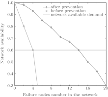
In order to verify the effectiveness of the control model, we compare the FTEL topologies before and after preventing cascading failure. In the experiments, in each round each node exchanges data to its neighboring nodes. In each round the nodes with energy depletion are removed. And the nodes are randomly removed according to the Poisson rule. The changes of the topology before and after prevention are shown in Fig. 1.
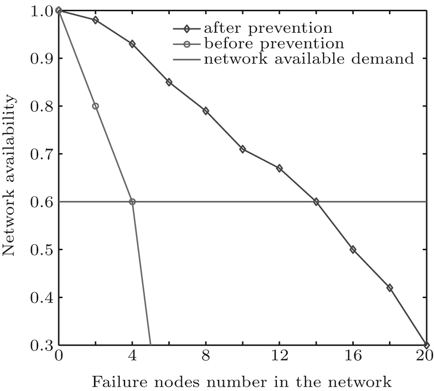 | Fig. 1. Comparison of the prevention effectiveness. |
The network availability requires that the network satisfies communication service. It varies with the actual condition. In Fig. 1, we can see that the network availability after preventing cascading failure is much better than the topology before prevention. When the network availability is 0.6, the topology before preventing cascading failure can only tolerate 5 failure nodes and the topology after preventing cascading failure can tolerate 14 failure nodes. It is due to the fact that in the topology before preventing cascading failure, a failure of one node can cause the failure of the other nodes due to load changes. While in the topology after preventing cascading failure, a failure of one node will not affect other nodes due to the control method for cascading failure. Therefore, the control method for cascading failure is effective.
We have shown the effectiveness of the control model for cascading failure. Now, we will study the performance of network after preventing cascading failure. The network lifetime and fault tolerance are important performances of the network. Here, we study the network lifetime and fault tolerance of the topology after preventing cascading failure.
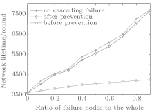
In this experiment, the lifetime of WSNs is the time when the first node in the network fails. Here, we compared the lifetime of FTEL topologies before preventing cascading failure, after preventing cascading failure and without cascading failure. The three topologies are running, respectively. And a percentage of the nodes are removed. Then we observe the remaining network lifetime, as shown in Fig. 2</p>
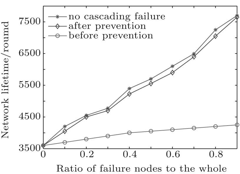 | Fig. 2. Comparison of the lifetime of the WSNs. |
Figure 2 shows that the lifetime of the topology after preventing cascading failure is smaller than the topology with no cascading failure. That is because the control model for cascading failure consumes a part energy of nodes. From Fig. 2, we can also obtain that the lifetime of the topology after preventing cascading failure is much longer than the topology before preventing cascading failure. It shows that the control method for cascading failure can effectively reduce the influence of cascading failure on the network performance.
In the experiments, random failure is regarded as the process that the nodes are removed randomly in the network, and selective failure is regarded as the process that the nodes are removed selectively according to the node degree descending.
Figure 3 shows the random failure tolerance of the three topologies before preventing cascading failure, after preventing cascading failure and without cascading failure. The corresponding relationship between the largest connected component scale and the random failure node radio is also shown. From Fig. 3, we can find that when the same number of random failure nodes are removed, the network scale of the topology without cascading failure and the topology after preventing cascading failure are similar. That is, almost no cascading failure occurs in the topology after preventing cascading failure. And the network scale of the two topologies are larger than the topology before preventing cascading failure. It indicates that the control model for cascading failure can make the network still have well fault tolerance for random failure.
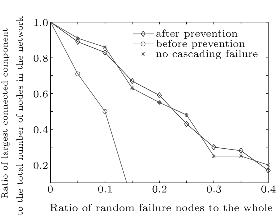 | Fig. 3. Comparison of the topology random failure tolerance. |
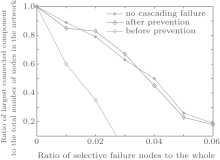
Figure 4 shows the changes of the largest connected component scale with the selective failure node radio for the three topologies without cascading failure, before preventing cascading failure and after preventing cascading failure. As shown in Fig. 4, when the same number of nodes are removed selectively, the network scale of the topologies without cascading failure and after preventing cascading failure are larger than the topology before preventing cascading failure. Therefore, the topology with the control model for cascading failure can still keep well fault tolerance for selective failure.
 | Fig. 4. Comparison of the topology selective failure tolerance. |
In this paper, for the large-scale cascading failure problems of the scale-free topology in WSNs, cascading failure of the scale-free topology of WSNs is studied and a control method for the cascading failure is proposed. Through analyzing the cascading failure of scale-free topology of WSNs, we build the cascading failure model of scale-free topology in WSNs. Based on the cascading failure model, the critical load triggering the larger-scale cascading failure is obtained. In addition, in the operation process of network, the actual load on the node is obtained by analyzing the characteristics of the data traffic distribution. Then the actual load on the node is less than the corresponding critical load, and the large-scale cascading failure can be prevented. Experimental tests demonstrate the effectiveness of the control method, and verify that the topology after preventing cascading failure by the control method still has well performance. The control method proposed in this paper is applied to the type of scale-free fault tolerant topology in WSNs in which the relay nodes with redundant links can be deleted. In our future research, we will study the effective control method by applying common fault tolerant topology on the basis of the critical node load and the actual node load.
| 1 |
|
| 2 |
|
| 3 |
|
| 4 |
|
| 5 |
|
| 6 |
|
| 7 |
|
| 8 |
|
| 9 |
|
| 10 |
|
| 11 |
|
| 12 |
|
| 13 |
|
| 14 |
|
| 15 |
|
| 16 |
|
| 17 |
|
| 18 |
|
| 19 |
|
| 20 |
|
| 21 |
|
| 22 |
|
| 23 |
|
| 24 |
|