


Three-dimensional spin–orbit coupled Fermi gases: Fulde–Ferrell pairing, Majorana fermions, Weyl fermions, and gapless topological superfluidity*
[Liu Xia-Jia) , Hu Huia) , Pu Hanb), c)†  ]
]
]
|
|


†Corresponding author. E-mail: hpu@rice.edu
*Project supported by the ARC Discovery Projects (Grant Nos. FT140100003, FT130100815, DP140103231, and DP140100637), the National Basic Research Program of China (Grant No. 2011CB921502), the US National Science Foundation, and the Welch Foundation (Grant No. C-1669).
We theoretically investigate a three-dimensional Fermi gas with Rashba spin–orbit coupling in the presence of both out-of-plane and in-plane Zeeman fields. We show that, driven by a sufficiently large Zeeman field, either out-of-plane or in-plane, the superfluid phase of this system exhibits a number of interesting features, including inhomogeneous Fulde–Ferrell pairing, gapped or gapless topological order, and exotic quasi-particle excitations known as Weyl fermions that have linear energy dispersions in momentum space (i.e., massless Dirac fermions). The topological superfluid phase can have either four or two topologically protected Weyl nodes. We present the phase diagrams at both zero and finite temperatures and discuss the possibility of their observation in an atomic Fermi gas with synthetic spin–orbit coupling. In this context, topological superfluid phase with an imperfect Rashba spin–orbit coupling is also studied.
Quantum simulations of intriguing many-body problems with ultracold atoms have now become a paradigm in different fields of physics.[1] The major advantage of ultracold atoms is their unprecedented controllability in tuning interactions, dimensionality, populations, and species of atoms, which constitute an ideal toolbox for understanding the consequence of strong interactions.[2] Most recently, a new tool — a synthetic non-Abelian gauge field or spin– orbit coupling — was added to the toolbox.[3] In condensed matter physics, it is well known that spin– orbit coupling plays a key role in new-generation solid-state materials such as topological insulators, [4, 5] quantum spin Hall systems, [6] and non-centrosymmetric superconductors.[7] In this respect, recent realization of synthetic spin– orbit coupling in ultracold atoms opens up an entirely new direction to quantum simulate and characterize these new-generation materials, without the need to overcome the intrinsic complexibility in compositions and interactions, which is often encountered in solid-state systems.
Indeed, over the past few years, a tremendous amount of theoretical works along this direction has already been seen[8– 50] triggered by the demonstration of a particular spin– orbit coupling in ultracold atomic Fermi gases by the two-photon Raman technique, which has an equal superposition of Rashba and Dresselhaus spin– orbit couplings.[51– 54] In previous studies, the possibility of observing a peculiar two-body bound state and the related anisotropic superfluid induced by Rashba spin– orbit coupling was discussed.[11, 13, 14] In the presence of an out-of-plane Zeeman field, the routine to a topological superfluid and Majorana fermions in two dimensions[12, 17, 21, 26, 55] or to a Weyl superfluid in three dimensions, [15, 34, 56] which has exotic quasiparticles with linear energy dispersion in momentum space, was addressed. Later on, it was realized that unconventional Fulde– Ferrell pairing could be significantly enhanced by spin– orbit coupling in combination with an in-plane Zeeman field due to the distorted Fermi surface.[27– 33, 35, 42, 43] As a result, spin– orbit coupled Fermi gases provide an ideal candidate to investigate the long-sought Fulde– Ferrell superfluidity or superconductivity, [57] which is yet to be unambiguously confirmed in solid-state systems. Very recently, it was shown that the Fulde– Ferrell pairing may coexist with the topological order, leading to the predictions of topological Fulde– Ferrell superfluids, [38– 41, 48] including a brand-new quantum matter of gapless topological superfluid that has no analogies in solid-state systems.[44, 46, 50]
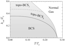
In this work, by using a spin– orbit coupled Fermi gas in three dimensions with both in-plane and out-of-plane Zeeman fields as a prototype, we show that the above-mentioned concepts in unconventional superfluid phases can be examined and demonstrated in near-future experiments. These unconventional phases include Fulde– Ferrell state — an exotic fermionic superfluid featuring Cooper pairs with finite center-of-mass momentum, Majorana fermions — a type of exotic quasiparticle mode that is its own anti-particle, Weyl fermions — particles with linear dispersion, i.e., their energy depends on their momentum linearly, and topological superfluidity — superfluids with nontrivial topological order. Our main result is summarized in Fig. 1, which displays a very rich phase diagram at zero temperature and at interaction parameter 1/(kFas) = − 0.5 and spin– orbit coupling strength λ = EF/kF, where kF and 
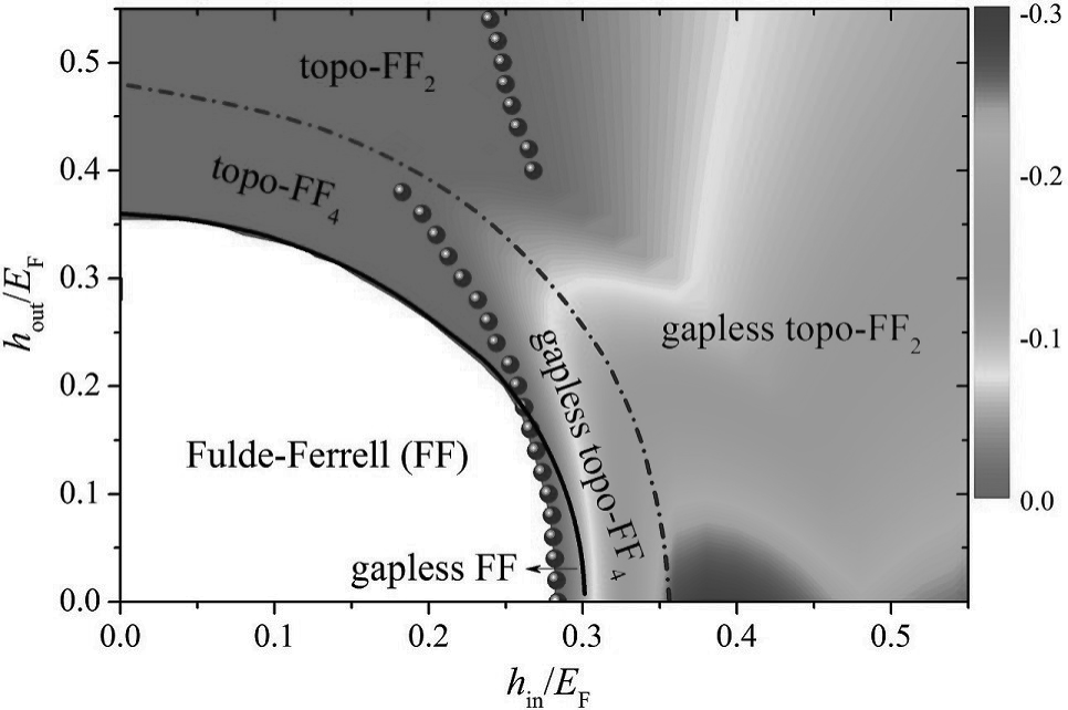 | Fig. 1. Zero temperature phase diagram of a 3D Rashba spin– orbit coupled Fermi gas on the plane of in-plane and out-of-plane Zeeman fields, with a spin– orbit coupling strength λ = EF/kF and an interaction strength 1/(kFas) = − 0.5. The color map shows the lowest energy in the lower particle branches in units of EF. There are various superfluid phases, as described in detail in the text. The solid line shows the topological phase transition. While the dot-dashed line indicates the transition within the two types of topological superfluids, which have four or two Weyl nodes/loops, respectively. The solid circles are the boundary where the superfluid becomes gapless, apart from the Weyl nodes. |
We note that the same Fermi system has been considered earlier by Xu et al. with the focus on the anisotropic Weyl fermions due to an in-plane Zeeman field.[45] Our results differ from theirs in several ways. (i) We clarify that the in-plane Zeeman field itself can drive a topological phase transition and lead to a gapless topological superfluid. (ii) In the topological phases, a Fulde– Ferrell superfluid, either gapped or gapless, can be further classified according to the number of Weyl nodes (in the gapped area) or Weyl loops (in the gapless region). With increasing Zeeman field, a topologically trivial phase first becomes a topo-FF4 and then turns into a topo-FF2 when the Zeeman field is sufficiently large; Majorana surface states in different superfluid phases are discussed. (iii) Various finite-temperature phase diagrams are presented, which are useful for future experiments that have to be carried out at non-zero temperatures. (iv) We consider an alternative form of spin– orbit coupling away from the Rashba limit and show that different intriguing topological phases do not depend critically on the type of spin– orbit coupling.
On the other hand, we also note that our theoretical investigations are based on the mean-field theory. The beyond mean-field effect has been recently considered by Zheng and co-workers[49] by using a pseudogap approximation for pair fluctuations.
Our paper is organized as follows. In the next section, we introduce the mean-field theoretical framework. In Section 3, we discuss in detail the conditions for different unconventional superfluid phases, their energy spectrum, and the surface states when a hard-wall potential is imposed at the (opposite) two boundaries. Finite temperature phase diagrams at different Zeeman fields are constructed. We also investigate how the zero-temperature phase diagram is affected by the form of spin– orbit coupling. Finally, Section 4 is devoted to the conclusions and outlooks.
We consider a three-dimensional (3D) spin-1/2 Fermi gas near a broad Feshbach resonance with two-dimensional (2D) spin– orbit coupling 


where 
and 

that describes the contact interaction between two atoms in different spin states with an interaction strength U0. In the above Hamiltonian, 

where V is the volume of the system. Experimentally, the scattering length as can be tuned precisely to an arbitrary value by sweeping an external magnetic field across the Feshbach resonance, [2] from the weakly interacting limit of Bardeen– Cooper– Schrieffer (BCS) superfluids to the strong-coupling limit of Bose– Einstein condensates (BEC).[58]
It is now widely known that spin– orbit coupling together with in-plane Zeeman field can induce the Fulde– Ferrell pairing, with an order parameter having a finite center-of-mass momentum along the direction of the in-plane Zeeman field.[27– 32] This finite-momentum pairing, also referred to as the helical phase, was first proposed in the study of noncentrosymmetric superconductors.[7, 59– 63] As we apply the in-plane Zeeman field along the z direction, we assume an order parameter

with an FF momentum q = qez, where ez is the unit vector along the z direction. Within the mean-field theory, we may approximate the interaction Hamiltonian as

For a Fermi superfluid, it is useful to introduce the following Nambu spinor to collectively denote the field operators:

where the first two and the last two field operators in Φ (x) could be interpreted as the annihilation operators for particles and holes, respectively. The total mean-field Hamiltonian can then be written in a compact form,
where the factor 1/2 in the last term arises from the redundant use of particle and hole operators in the Nambu spinor Φ (x). Accordingly, a zero-point energy 

Note that the spin– orbit coupling term in the hole sector of Eq. (9) does not change sign as spin– orbit coupling respects the time-reversal symmetry. The mean-field Hamiltonian Eq. (8) can be solved by taking the standard Bogoliugov transformation. In our case, it is more convenient to directly diagonalizing the Bogoliubov Hamiltonian

with the plane-wave quasiparticle wave-function
and quasiparticle energy Eη (k). Equation (11) explicitly shows how the FF momentum q = qez affects the quasiparticle wave-fucntions. The FF momentum can be roughly regarded as the center-of-mass momentum of the Cooper pairs. In a recent work, Jiang et al. studied the expansion dynamics of a quasi-1D spin– orbit coupled Fermi gas with FF pairing by solving the time-dependent version of the Bogoliubov– de Gennes equation, and showed that the FF pairing manifests itself in the displacement of the center-of-mass position of the whole cloud during time of flight.[48] As the Bogoliubov Hamiltonian now becomes a 4 × 4 matrix, the four eigenvalues and eigenstates can be collectively specified as η = {α , ν }, where the index α ∈ (1, 2) indicates the upper (1) or lower (2) band split by the spin– orbit coupling and Zeeman fields, and ν ∈ (+ , − ) stands for the particle (+ ) or hole (− ) branch. The ansatz of the wave-fucntion, Eq. (11), is inspired by the use of the Fulde– Ferrell order parameter as defined in Eq. (5) and is also consistent with the fact that the hole wave-function is a time-reversal partner of the particle wave-fucntion. By substituting Eq. (11) into the Bogoliubov equation (10), we obtain a 4 × 4 Bogoliubov matrix for [ukη ↑ ukη ↓ , vkη ↑ , vkη ↓ ]T, in which the operator 
and 

and 
where the zero-point energy (1/2)∑ kη Eη (k) in the square bracket is again due to the redundant use of particle and hole operators, and we have rewritten the zero-point energy
In the topological phase, the superfluid can support gapless surface states. To demonstrate this non-trivial consequence of topological order, we consider adding a hard-wall confinement in the x direction and calculate the resulting energy spectrum En(kz, ky). The zero-energy Majorana fermion modes are expected to appear at kz = 0 and at the two boundaries x = 0 and x = L, [4, 5, 55] where 
The use of a hard-wall potential means that the wave-function of quasiparticles along the x axis is no longer a plane wave, as the translation symmetry along that direction is broken. Neglecting the effect on the order parameter by the confinement, which is valid for sufficiently large L, we take the ansatz
By substituting Eq. (15) into Eq. (9), the resulting BdG Hamiltonian for a given set of (kz, ky) has the form

where
To diagonalize the BdG Hamiltonian Eq. (16), we expand all the quasiparticle wavefunctions in terms of the single-particle eigenstates of the hard-wall potential, which are given by

with l = 1, 2, 3, … . For example, for ukykz↑ (x) we have
where Nmax ≫ 1 is a high energy cut-off. This converts the BdG Hamiltonian Eq. (16) into a 4Nmax × 4Nmax symmetric matrix, with the matrix elements
and
The diagonalization leads directly to the energies En(ky, kz) and the wavefunctions of the quasiparticle states. The surface or edge modes can be easily identified as they are localized near the boundary at x = 0 or L. It turns out that the surface modes localized at opposite boundaries possess opposite momenta along the z axis, and hence can be regarded as chiral surface modes.
For a uniform Fermi gas, we use the natural units, 2m = ħ = kB = kF = EF = 1. This means that we take the Fermi wavevector kF and Fermi energy EF as the units for wavevector and energy, respectively. Thus, the spin– orbit coupling will be parameterized by the dimensionless parameter 


Moreover, we have the number equation

These equations are solved self-consistently by using Newton’ s gradient approach. The various derivatives can be approximated by numerical differences. The approach is very efficient, provided a good guess of the initial parameters, which may be obtained by plotting the contour plot of the mean-field thermodynamic potential. Throughout the paper, we focus on the BCS side with a dimensionless interaction parameter 1/(kFas) = − 0.5 and use the mean-field theory to solve the model Hamiltonian at both zero and finite temperatures. The spin– orbit coupling strength is always fixed to λ = EF/kF. In most cases, we consider a Rashba spin– orbit coupling. The deviation from the Rashba case will be investigated at the end of the section.
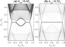
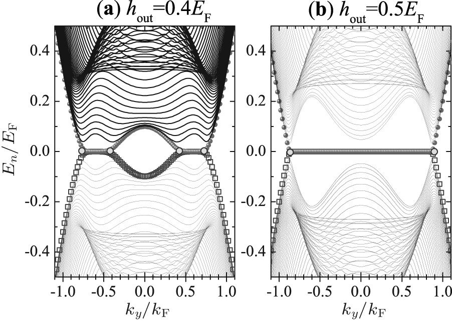
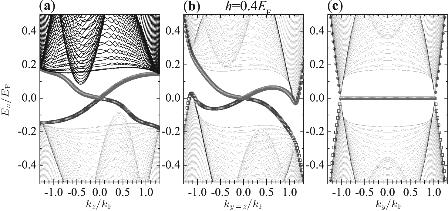
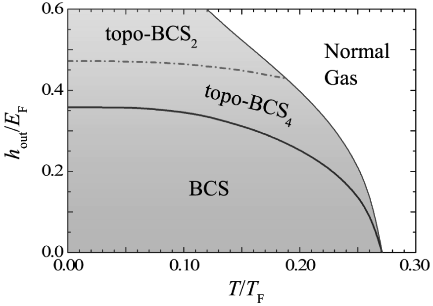
Let us first consider the simplest case with an out-of-plane Zeeman field only, a situation that was previously addressed by Gong and co-workers.[15] The zero-temperature phase diagram is reported in Fig. 2(a), together with the energy spectra of two topologically non-trivial phases at hout = 0.4EF and hout = 0.5EF in Figs. 2(b) and 2(c), respectively. The chiral surface states in the presence of a hard-wall confinement at the two boundaries along the x direction are shown in Fig. 3.
 | Fig. 2. (a) Evolution of the superfluid phase with increasing out-of-plane Zeeman field at zero in-plane Zeeman field hin = 0. The system evolves from a standard BCS superfluid to a topological non-trivially superfluid with either four (topo-BCS4) or two Weyl nodes (topo-BCS2). The solid and dashed lines show the energy at k = 0 [E2+ (k = 0)] and the minimum energy [minE2+ (k)] of the lower particle branch. Panels (b) and (c) show the characteristic quasiparticle excitation spectrum E2± (kx = 0, ky, kz) in the topo-BCS4 (hout = 0.4EF) and topo-BCS2 phases (hout = 0.5EF), respectively. We note that the spectrum is symmetric with respect to ky and we plot only the left part with ky ≤ 0. |
 | Fig. 3. Chiral surface modes (highlighted by blue empty squares and red solid circles) with a hard-wall confinement along the x direction at kz = 0, in the (a) topo-BCS4 or (b) topo-BCS2 phases. The system may be viewed as a stack of many 2D topological superfluids along the y direction. Accordingly, the surface modes of the system may be understood as a collection of the edge modes of these 2D systems. |
In the phase diagram, the properties of any possible 3D phase can be understood by dimensional reduction in momentum space to a set of 2D phases.[4, 56] The basic idea of dimensional reduction is to treat the 3D Hamiltonian, for example, 


each of which is described by an effective 2D Hamiltonian 
In the presence of an out-of-plane Zeeman field hout only, it is known that the 2D Hamiltonian

where 

whose value depends critically on ky. Due to a positive chemical potential μ on the BCS side, it is easy to see that the topological phase transition first occurs at 
By increasing the out-of-plane Zeeman field, the slices with 


From the above analysis, it is clear that the appearance of a topological phase with four and two Weyl nodes can be determined by the closing of the global energy gap and of the local energy gap at k = 0, respectively. This is demonstrated in Fig. 2(a), where we plot the minimum energy [min E2+ (k)] and the local energy at k = 0 [E2+ (k = 0)] of the lower particle branch by using the dashed and solid lines, respectively. Here we use the minimum energy, instead of a global energy gap Eg = 2|min E2+ (k)| that is the energy difference between the minimum energy of the particle branch and the maximum of the hole branch due to the particle– hole symmetry E2+ (k) = − E2− (− k). As we shall see below, the minimum energy is more useful to characterize the emergence of a gapless phase.[44] With increasing the out-of-plane Zeeman field, the minimum energy develops a zero-energy plateau as the system enters the topological phase due to the occasional band touching of the particle and hole branches at the Weyl nodes. In contrast, the local energy at k = 0 will close and then reopen at the critical field where the number of Weyl nodes decreases from four to two.
In the topological phase, the formation of isolated Weyl nodes can be clearly identified in the energy spectrum in momentum space, as shown in Figs. 2(b) and 2(c). It is interesting that these Weyl nodes are connected continuously by zero-energy Majorana surface states once we impose the hard-wall confinement at the two boundaries along the x direction (see Fig. 3). The existence of the Majorana modes is easy to understand from the dimensional reduction mentioned earlier: the surface states with a given ky and kz of the 3D Hamiltonian
To close this subsection, we note that, with a small in-plane Zeeman field, the phase diagram is essentially unchanged. The only difference is that Cooper pairs now acquire a finite center-of-mass momentum. The resulting topologically nontrivial phases are better referred to as topo-FF4 or topo-FF2, according to the number of Weyl nodes. The linear quasiparticle spectrum around a Weyl node becomes anisotropic.[45] In the presence of a large in-plane Zeeman field, however, the phase diagram would change qualitatively, as we now turn to discuss in great detail.
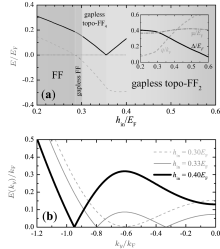
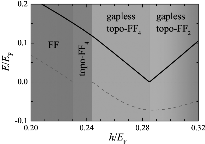
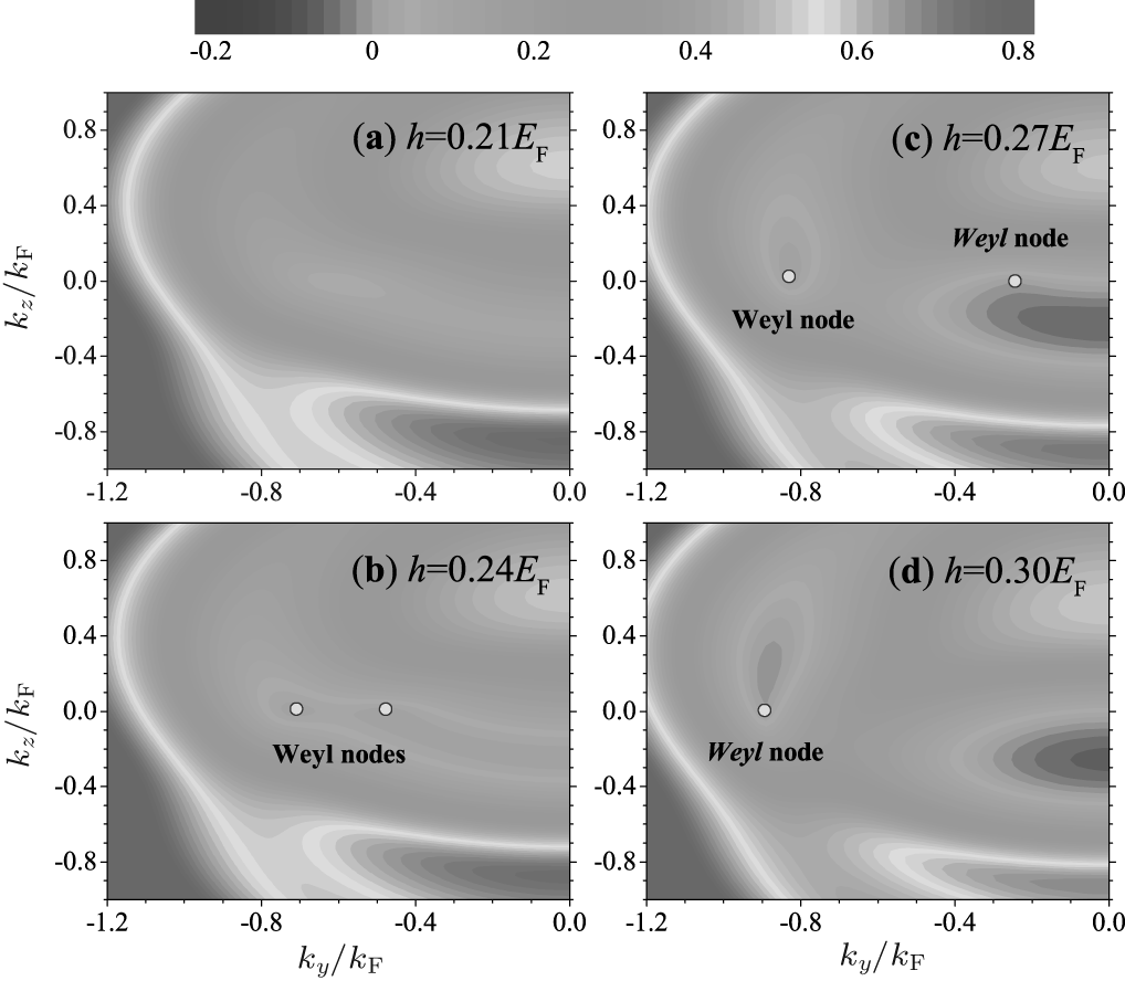
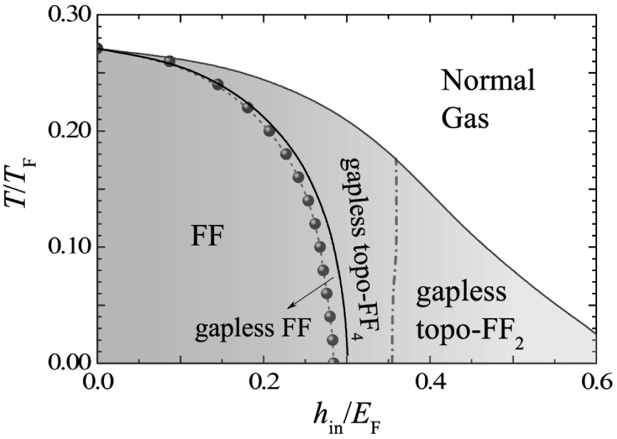
Figure 4(a) reports the phase diagram in the presence of an in-plane Zeeman field only. Compared with Fig. 2, with increasing Zeeman field strength, the local energy at k = 0 (solid line) shows similar behavior. By contrast, the minimum energy minE2+ (k) (dashed line) exhibits very different field dependence. It becomes negative at 
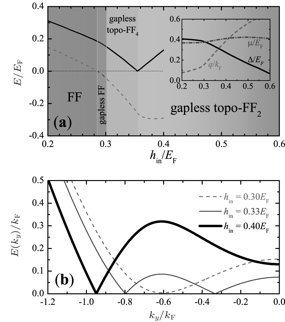 | Fig. 4. (a) Evolution of the superfluid phase with increasing in-plane Zeeman field at zero out-of-plane Zeeman field hout = 0. Driven by the in-plane field only, the system evolves from a gapped FF superfluid to a gapless FF state, and then to a topologically non-trivial FF superfluid with either four (gapless topo-FF4) or two Weyl nodes/loops (gapless topo-FF2). The solid and dashed lines show the energy at k = 0 [E2+ (k = 0)] and the minimum energy [minE2+ (k)] of the lower particle branch. The inset shows the chemical potential, pairing gap and FF pairing momentum as a function of the in-plane Zeeman field. (b) The energy of the lower particle branch along the ky direction, E2+ (kx = 0, ky, kz = 0), at hin/EF = 0.30 (gapless FF, dashed line), 0.33 (gapless topo-FF4, thin solid line), and 0.40 (gapless topo-FF2, thick solid line). The minimum energy touches zero at the positions of Weyl nodes. |
Our answer is yes, after a careful check on the structure of the energy spectrum (Fig. 5) as well as the appearance of the Majorana surface states (Fig. 6). The energy spectrum can have Weyl nodes as the in-plane Zeeman field 


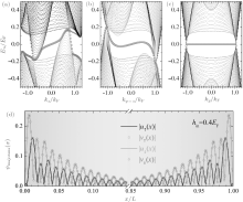
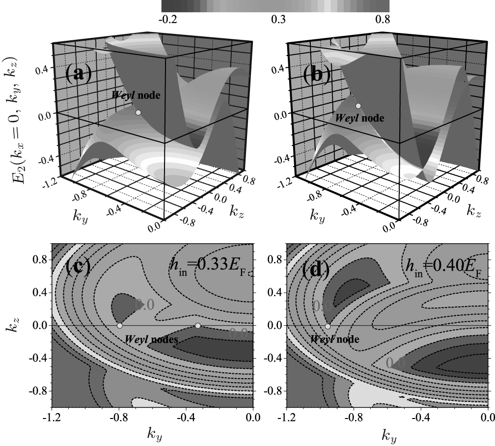 | Fig. 5. The characteristic quasiparticle excitation spectrum E2± (kx = 0, ky, kz) in the gapless topo-FF4 phase with hin = 0.33EF (a) and in the gapless topo-FF2 phase with hin = 0.40EF (b). The corresponding contour plots of E2+ (kx = 0, ky, kz) are shown in panels (c) and (d), respectively. The Weyl nodes are highlighted by yellow solid circles. We note that the out-of-plane Zeeman field hout = 0. The spectrum is symmetric with respect to ky, so we plot only the left part with ky ≤ 0. |
In Figs. 6(a)– 6(c), we present the energy dispersion of the surface states in the gapless topo-FF2 phase. At kz = 0 (Fig. 6(c)), we observe the same Majorana flat band as in the case of out-of-plane Zeeman field (see, for example, Fig. 3(b)), which connects the two Weyl nodes in the bulk spectrum. To confirm that the zero-energy surface states are indeed Majorana modes, we plot the wave-function of one of the surface states at ky = kz = 0 in Fig. 6(d). The wave-function is well localized at the two boundaries and satisfies the desired symmetry 
 | Fig. 6. Majorana surface modes with a hard-wall confinement along the x direction in the gapless topo-FF2 phase (hin = 0.4EF), at (a) ky = 0, (b) along the ky = kz line, or (c) at kz = 0. The wave-functions of the Majorana mode at ky = kz = 0 are shown in panel (d), which are well localized near the two boundaries x = 0 and  |
Our results of in-plane Zeeman field induced gapless topological superfluids are not captured by a previous study based on the same model Hamiltonian.[45] In that work, in the absence of an out-of-plane Zeeman field, the system was thought to always be in the gapless Fulde– Ferrell superfluid.[45] This discrepancy may originate from a different definition of topological phase for the 2D slices, in the point of view of dimensional reduction. On the other hand, we are not able to produce the contour plot of the zero-energy quasiparticle spectrum at a large in-plane Zeeman field, as shown by the blue line in Fig. 2(b) of Ref. [45], which has connected closed lines for nodal points and therefore was considered topologically trivial. The contour plots in Figs. 5(c) and 5(d) are rather similar to the one with a small out-of-plane Zeeman field shown by the red line in Fig. 2(b) of Ref. [45], which was also regarded by the authors as topologically non-trivial.
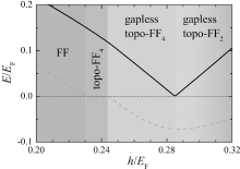
We now consider another special case with equal in-plane and out-of-plane Zeeman fields. Figure 7 shows the phase diagram determined by monitoring the minimum energy and the local energy at k = 0 of the lower particle branch. The contour plots of the energy spectrum at kx = 0 in different superfluid phases are reported in color in Fig. 8. A gapped topological Fulde– Ferrell phase can be easily identified from the zero-energy plateau in the minimum energy. A close look at the energy spectrum (Fig. 8(b)) indicates that this phase has four Weyl nodes and therefore should be classified as a topo-FF4 phase. With increasing Zeeman field, nodal points develop in the energy spectrum and the system enters the gapless topological phase with four (Fig. 8(c)) and then two Weyl nodes (Fig. 8(d)).
 | Fig. 7. (a) Evolution of the superfluid phase with equally increasing in-plane and out-of-plane Zeeman fields (i.e., hin = hout = h). The system evolves from a gapped FF superfluid to a gapped topologically nontrivial topo-FF4 state, and then to a gapless topologically non-trivial FF superfluid with either four (gapless topo-FF4) or two Weyl nodes/loops (gapless topo-FF2). The solid and dashed lines show the energy at k = 0 [E2+ (k = 0)] and the minimum energy [minE2+ (k)] of the lower particle branch. |
 | Fig. 8. Contour plots of the particle branch E2+ (k) in (a) the gapped FF phase, (b) the gapped topo-FF4 phase, (c) the gapless topo-FF4 phase, and (d) the gapless topo-FF2 phase. The Weyl nodes are highlighted by yellow solid circles. We note that the in-plane and out-of-plane Zeeman fields are equal, hin = hout = h. The spectrum is symmetric with respect to ky, so we plot only the left part with ky ≤ 0. |
In Fig. 9, we show the Majorana surface modes in the gapless topo-FF2 phase with hin = hout = 0.4EF. Along the cut kz = 0 as shown in Fig. 9(c), we again find the Majorana flat band as a function of the parameterized momentum ky. This is indeed a very robust feature of our system as the Hamiltonian is dispersionless along the ky axis. When we make cuts along other directions, i.e., along the ky = 0 and ky = kz axis in Figs. 9(a) and 9(b), the surface states do have dispersion. They propagate along opposite directions at the two boundaries, as a result of the gapped energy spectrum along the cuts, [44] although the topological phase itself is globally gapless in the bulk.
 | Fig. 9. Chiral surface modes with a hard-wall confinement along the x direction in the gapless topo-FF2 phase (hin = hout = 0.4EF), at (a) ky = 0, (b) along the ky = kz line, or (c) at kz = 0. |
By tuning in-plane and out-of-plane Zeeman fields, we obtain the zero-temperature phase diagram, as displayed earlier in Fig. 1. The solid line, which separates a usual Fulde– Ferrell superfluid from a topologically non-trivial Fulde– Ferrell superfluid, is determined by the first appearance of Weyl nodes in the energy of the lower particle branch along the ky direction, E2+ (kx = 0, ky, kz = 0) (see, for example, Fig. 4(b)). The transition within different topological phases (i.e., from four to two Weyl nodes), shown by the dot-dashed line, can be conveniently determined by the closing of the local energy gap at origin, i.e., E2+ (k = 0) = 0. On the other hand, the gapless transition indicated by red solid circles in the figure could be obtained from the critical field at which the minimum energy min E2+ (k) becomes negative. It is worth noting that the red solid circles are not smoothly connected. Physically, to the left of these solid circles, the topological phase has occasionally touched Weyl nodes along the ky axis; while to the right of the solid circles, each Weyl node extends to form a loop of nodal points on the ky– kz plane, as we already discussed in Figs. 5(c) and 5(d).
It is impressive that on the BCS side, the topological Fulde– Ferrell phases, either gapped or gapless, dominate in the phase diagram. In particular, the gapless topological Fulde– Ferrell superfluid with two Weyl nodes is already energetically favorable at a moderately large in-plane Zeeman field (i.e., hin > 0.35EF).
In current cold-atom experiments, the lowest accessible temperature is about 0.05– 0.1TF.[66] It is thus useful to consider how the different superfluid phases evolve as temperature increases. The calculation proceeds in a similar way as the zero-temperature case. The only difference here is that the thermodynamic potential Ω mf is modified as a finite T affects the last term on the right hand side of Eq. (14). In Figs. 10– 12, we show the finite-temperature phase diagrams at different configurations of Zeeman fields. Our mean-field theory is less reliable at finite temperature. However, on the BCS side with a weak interaction parameter 1/(kFas) = − 0.5, we anticipate that it will provide a very good qualitative description.
 | Fig. 10. Finite-temperature phase diagram on the T– hout plane at zero in-plane Zeeman field hin = 0. |
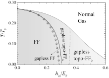
 | Fig. 11. Finite-temperature phase diagram on the hin– T plane at zero out-of-plane Zeeman field hout = 0. |
 | Fig. 12. Finite-temperature phase diagram on the h– T plane with equal in-plane and out-of-plane Zeeman fields hin = hout = h. |
In the presence of an out-of-plane Zeeman field only (Fig. 10), the finite-temperature phase diagram has been earlier discussed by Seo and co-workers.[34] It contains two topological BCS phases and is relatively easy to understand. In the other two cases with in-plane Zeeman field only (Fig. 11) and equal in-plane and out-of-plane Zeeman fields (Fig. 12), gapless topological Fulde– Ferrell superfluids emerge at a sufficiently large field strength. It is remarkable that the phase space for these gapless topological superfluids is very significant at finite temperature. In particular, when the system is cooled down from a normal state at high temperature, the pairing instability first occurs towards the formation of gapless topological phases. The typical superfluid transition temperature is about 0.15TF, which is clearly within reach in current cold-atom experiments.[66]
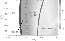
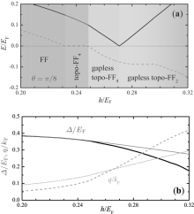
We now turn to consider a general form of spin– orbit coupling with λ z = λ cosθ and λ x = λ sinθ , away from the Rashba spin– orbit coupling that corresponds to θ = π /4. This investigation is helpful for future experiments, as the synthetic spin– orbit coupling realized in cold-atom experiments may not acquire the perfect form of Rashba spin– orbit coupling. In Fig. 13, we show the evolution of the zero-temperature phase diagram as a function of the angle θ down to θ = π /8 in the presence of equal in-plane and out-of-plane Zeeman fields. The Zeeman field dependence of the minimum energy min E2+ (k) and the local energy at k = 0 E2+ (k = 0) of the lower particle branch in the case of θ = π /8, where the component of Dresselhaus spin– orbit coupling becomes significant, are reported in Fig. 14(a).
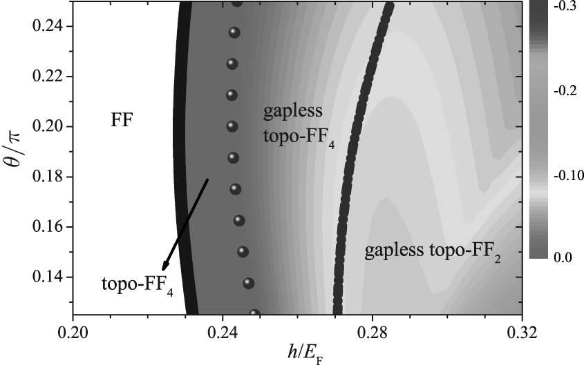 | Fig. 13. Zero-temperature phase diagram with an anisotropic spin– orbit coupling  |
 | Fig. 14. (a) Evolution of the superfluid phase with equally increasing in-plane and out-plane Zeeman fields, and with an imperfect Rashba spin– orbit coupling at the angle θ = π /8. The system evolves from a gapped FF superfluid to a gapped topologically nontrivial topo-FF4 state, and then to a gapless topologically non-trivial FF superfluid with either four (gapless topo-FF4) or two Weyl nodes/loops (gapless topo-FF2). The solid and dashed lines show the energy at k = 0 [E2+ (k = 0)] and the minimum energy [minE2+ (k)] of the lower particle branch. (b) The pairing gap (solid line) and FF pairing momentum (dashed line) as a function of the Zeeman field. The thick and thin lines correspond to the cases with θ = π /8 and θ = π /4, respectively. |
The phase diagram is less affected by tuning the form of spin– orbit coupling. With decreasing θ , the phase space for the topological phases (including gapped or gapless topo-FF4, and gapless topo-FF2) is essentially unchanged. It is remarkable that the most interesting gapless topo-FF2 phase seems to be more favorable away from the Rashba spin– orbit coupling. This could be attributed to the increasing Fulde– Ferrell momentum q at large Zeeman fields, as shown in Fig. 14(b), which favors the gapless phase and also the topological phase with two Weyl nodes.
We have presented a systematic investigation of the superfluid phases of a spin– orbit coupled Fermi gas with both in-plane and out-of-plane Zeeman fields, by using a dimensional reduction picture.[56] Driven by large Zeeman fields, in particular, the large in-plane Zeeman field, the system supports a number of intriguing features including Fulde– Ferrell pairing, topological superfluids with Majorana fermions in real space and Weyl fermions in momentum space, and also novel gapless topological superfluids. We have considered the phase diagram at both zero temperature and finite temperature. We have mainly focused on Rashba spin– orbit coupling. The case with an imperfect Rashba spin– orbit coupling has also been addressed, from a realistic experimental point of view. Our work complements the earlier investigation by Xu and co-workers[45] by providing a more complete phase diagram at zero temperature and extending the phase diagram to the case of finite temperature and with more general spin– orbit coupling.
In future studies, it will be useful to consider the pair fluctuations which become very significant at the BEC– BCS crossover at both zero and finite temperatures. The finite-temperature pair fluctuations for our system have been recently addressed within a pseudogap theory.[49] More rigorous treatments could rely on the different many-body T-matrix theories within the ladder approximation.[67, 68]
| 1 |
|
| 2 |
|
| 3 |
|
| 4 |
|
| 5 |
|
| 6 |
|
| 7 |
|
| 8 |
|
| 9 |
|
| 10 |
|
| 11 |
|
| 12 |
|
| 13 |
|
| 14 |
|
| 15 |
|
| 16 |
|
| 17 |
|
| 18 |
|
| 19 |
|
| 20 |
|
| 21 |
|
| 22 |
|
| 23 |
|
| 24 |
|
| 25 |
|
| 26 |
|
| 27 |
|
| 28 |
|
| 29 |
|
| 30 |
|
| 31 |
|
| 32 |
|
| 33 |
|
| 34 |
|
| 35 |
|
| 36 |
|
| 37 |
|
| 38 |
|
| 39 |
|
| 40 |
|
| 41 |
|
| 42 |
|
| 43 |
|
| 44 |
|
| 45 |
|
| 46 |
|
| 47 |
|
| 48 |
|
| 49 |
|
| 50 |
|
| 51 |
|
| 52 |
|
| 53 |
|
| 54 |
|
| 55 |
|
| 56 |
|
| 57 |
|
| 58 |
|
| 59 |
|
| 60 |
|
| 61 |
|
| 62 |
|
| 63 |
|
| 64 |
|
| 65 |
|
| 66 |
|
| 67 |
|
| 68 |
|