Nonlinear partial differential equations are useful in describing various phenomena in applied mathematics and physics. Analytical solutions of these equations are usually not available, especially when the nonlinear terms are involved. Since only limited classes of the equations are solved by analytical means, numerical solutions of these nonlinear partial differential equations are of practical importance (see Refs.  [1]– [5]). Solitary waves are wave packets or pulses, which propagate in nonlinear dispersive media. Due to the dynamical balance between the nonlinearity and the dispersive effects, these waves retain a stable waveform. A soliton is a very special type of a solitary wave, which propagates without any change of its shape and velocity properties after collisions with other solitons. The present work is concerned with the numerical solution of the regularized long wave (RLW) equation, which was first derived by Peregrine to define undular bore development.^[6] Since then, this equation has been used to model a large number of problems arising in various areas of applied science. The RLW equation is an alternative description of nonlinear dispersive waves to the more usual Korteweg– de Vries (KdV) equation. It has been found to have solitary wave solutions and govern a large number of important physical phenomena such as nonlinear transverse waves in a shallow water, ion-acoustic, magneto-hydrodynamic waves in plasma and phonon packets in nonlinear crystals, anharmonic lattices, longitudinal dispersive waves in elastic rods, pressure waves in liquid– gas bubble mixtures, rotating flow down a tube, the lossless propagation of shallow water waves, and thermally exited phonon packets in low-temperature and nonlinear crystals.^{[7– 9]} Indeed, the RLW equation is a special case of the generalized regularized long wave (GRLW) equation, which is given by

where p is a positive integer, , ε and μ are positive constants which require the boundary conditions u → 0 as x → ± ∞ . It was proposed many years ago as a model for small-amplitude long waves on the surface of water.^{[6, 10]} Here the cases p = 1, 2 correspond to the RLW and MRLW equations, respectively.

The solutions of this kind of equations are important in many applications. However, for more general initial conditions, the theoretical solutions for these equations are limited. Therefore, many researchers have put in a great deal of effort to compute the solutions of these equations using various numerical methods and the numerical solutions of the initial and initial-boundary problems of the nonlinear GRLW equation.

Bona et al.^[11] investigated the Fourier spectral method for the initial value problem of the GRLW equation. The method of lines based on the discretization of the spatial derivatives by means of Fourier pseudo-spectral approximations for the GRLW equation was derived by Durá n and Ló pez– Marcos.^[12] Djidjeli et al.^[13] discussed a linearized implicit pseudo-spectral method for the RLW equation. Adomian decomposition method was implemented for finding the solitary-wave solutions of GRLW equation by Kaya and El. Syed.^{[14, 15]} Zhang^[16] developed an implicit second-order accurate and stable energy preserving finite difference method based on the use of central difference equations for the time and space derivatives for GRLW equation. A numerical method for the GRLW equation using a reproducing kernel function was studied by Xie et al.^[17] Jafari et al.^[18] used sine– cosine and tanh methods to obtain the solutions of the GRLW equation. Mokhtari and Mohammadi^[19] presented a mesh-free technique based on sinc basis functions for the numerical solution of the GRLW equation. In addition, they proposed a new iterative algorithm for solving the GRLW equation.^[20] Feng et al.^[21] presented a mesh-less method for the nonlinear GRLW equation based on the moving least-squares approximation. The GRLW equation is solved numerically via the Petrov– Galerkin method by Roshan.^[22] Their method uses a linear hat function as the trial function and a quintic B-spline function as the test function. Lin^[23] presented a numerical method based on parametric adaptive cubic spline functions for solving the GRLW equation.

The RLW equation is an important equation in physics media describing phenomena with weak nonlinearity and dispersion waves.^[24] Recently, many well-known numerical techniques, such as finite element methods based on the least square principle, ^{[25– 27]} finite element methods based on the Galerkin and collocation principles, ^{[28– 36]} the Petrov– Galerkin method, ^[37] the radial basis functions collocation method, ^{[38, 39]} B-spline differential quadrature methods, ^[40] mesh-less methods, ^[41] Galerkin and collocation methods, ^{[42– 45]} the spectral method^[46] and non-polynomial spline method^[47] are employed to solve the RLW equation.

The RLW equation possesses only three invariant constants of motion corresponding to conservation of mass, momentum, and energy given by^[48]

The MRLW equation is another particular case of the GRLW equation for p = 2. Gardner et al.^[48] used a collocation method with quintic B-splines for the numerical solution of the MRLW equation. Khalifa et al.^[49] applied a finite difference method to study solitary waves for the MRLW equation, and showed that the scheme is marginally stable. The MRLW equation is solved numerically via a collocation method using cubic B-splines finite element by Khalifa et al.^[50] Khalifa et al.^[51] used the Adomian decomposition method for solving the MRLW equation. Ali^[52] has developed a classical radial basis function collocation method for solving the MRLW equation. Raslan^[53] used the quadratic B-spline function and a central difference operator for the time derivative to develop a new algorithm based on the collocation method to solve the MRLW equation. A computational comparison study of quadratic, cubic, quartic, and quintic splines for solving the MRLW equation is presented by Raslan and Hassan.^[54] Raslan and EL-Danaf^[55] used the B-spline finite element method to solve the MRLW equation. The numerical scheme based on the quartic B-spline collocation method is designed for the numerical solution of the MRLW equation by Haq et al.^[56] Achouri and Omrani^[57] used the homotopy perturbation method to implement the MRLW equation with some initial conditions. The MRLW equation, with some initial conditions, is solved numerically via a variational iteration method by Labidi and Omrani.^[58] Dereli^{[59, 60]} simulated traveling wave solutions of the MRLW equation using the mesh-less method based on collocation with well-known radial basis functions. Khan et al.^[61] employed the homotopy analysis method to obtain an approximate numerical solution of the MRLW equation with some specified initial conditions. Karakoc et al.^[62] obtained a numerical solution of the MRLW equation based on the quintic B-spline collocation method over the finite elements.

The MRLW equation also has three conservation laws related to mass, momentum, and energy^[49]

The spline function is a piecewise continuous polynomial function suitable to approximate an arbitrary function. It is known to approximate an arbitrary function better than other polynomial functions with the same degree. Spline functions are used in many applications such as interpolation, data fitting, and numerical solution of ordinary and partial differential equations. Rashidinia and Mohammadi^{[63, 64]} derived approximate expressions for the dispersion relation of the nonlinear Klein– Gordon and sine– Gordon equations in the case of strong nonlinearities using a method based on tension spline functions and finite difference approximations. Also, Mohammadi developed explicit methods using exponential spline functions and finite difference approximations for the numerical solution of the generalized Burgers’ – Fisher, ^[65] convection– diffusion, ^[66] nonlinear Schrö dinger, ^[67] and Euler– Bernoulli beam^[68] equations. Chegini et al.^[47] employed non-polynomial spline basis functions to obtain approximate solutions of the RLW equation. Bian^[69] used the Crank– Nicolson (C– N) method combined with a B-spline basis set for time-dependent and time-independent calculations of the photoionization cross sections of atoms and molecules.

In this work, we use exponential B-spline collocation and Crank– Nicolson methods for the numerical study of the GRLW equation. Our main objective is to improve the accuracy of the cubic B-spline method by utilizing some parameters, which enable us to obtain various classes of methods. Our method is a modification of the cubic B-spline method for the numerical solution of Eq.  (1). Application of our method is simple. While solving initial boundary value problems in partial differential equations, the procedure is to combine a spline approximation for the space derivative with a Crank– Nicolson finite difference approximation for the time derivative. The combination of a finite difference and an exponential spline functions technique provides better accuracy than finite difference methods. Therefore, the time derivative is replaced by a finite difference representation and the space derivatives by exponential B-splines. We use the exponential B-spline basis that leads to the tri-diagonal nonlinear system which can be solved by well known algorithms such as the Newton algorithm. Numerical examples are presented, which demonstrate that the present scheme with exponential B-splines gives more accurate approximations than the scheme using cubic B-splines. Our method is a user friendly, economical and stable method for GRLW equation.

The rest of this article is organized as follows. In Section 2, the B-spline basis for the space of exponential splines is given and some interpolation results for exponential splines are stated. In Section 3, the construction of the exponential B-spline collocation method for the numerical solution of GRLW equation is described. In Section 4, the stability analysis is theoretically discussed. Using the Von Neuman method, the proposed method is shown to be unconditionally stable. Section 5 is devoted to the convergence analysis of our presented method. The method is shown to have second-order convergence. In Section 6, numerical examples are included to illustrate the practical implementation of the proposed method. The accuracy performance of the obtained numerical results are compared to the exact solution and other existing methods. The numerical results show that our proposed method is a promising approach for solving different types of these non-linear partial differential equations problems. Finally, we conclude our paper in Section  7.

For an interval [a, b], we divide it into n subintervals [x_i, x_{i + 1}] (i = 0, 1, … , n – 1) by the equidistant knots x_i = a + ih (i = 0, 1, … , n), where h = (b – a)/n.

A function of class is a piecewise non-polynomial, which interpolates a function u(x) at the mesh points x_i, depends on a parameter ρ and reduces to cubic spline in [a, b] as ρ → 0, called an exponential spline function. For more details about exponential spline functions and their definitions, we refer readers to Refs.  [66], [70], and [71] and the references therein.

Among various classes of splines, the polynomial spline has received great attention primarily because it admits a basis of B-splines which can be accurately and efficiently computed. It has been shown that an exponential spline also admits a basis of B-splines which can be defined as follows. Let B_i(x) be the B-spline centered at x_i and have a finite support on the four consecutive intervals . According to Ref.  [72], the B_i(x) can be defined as

where

and

Each basis function B_i(x) is twice continuously differentiable.

Let s(x) be the cubic spline and be the exponential spline. Now we consider the following results, which have been established by Pruess.^[73]

Theorem 1  .

Following Ref.  [74] we obtain the following theorem.

Theorem 2  .

These theorems together with the de Boor– Hall error estimate^[75] lead to the following corollary.

Corollary 1 if u(x, t) ∈ C⁴[a, b], then there exists a constant, χ _i, independent of h such that

In this section, we consider the initial-boundary value problem of the GRLW equation

with the initial condition

and the boundary conditions

where F(u, u_x) = ε u^pu_x, γ , ε , and μ are positive parameters, and ϕ (x), f₀(t), and f₁(t) are known functions.

The domain [a, b] × [0, T] is divided into an n × m mesh, with and , respectively. x_i = a + ih, for i = 0, 1, 2, … , n is the ith node. In the temporal dimension, the uniform step size k is used, so t_j = jk, j = 0, 1, … , m, is the time level for the jth step. The quantity U(x_i, t_j) represents the exact solution at (x_i, t_j) while u(x_i, t_j) represents the numerical solution at (x_i, t_j).

For stability analysis, following Refs.  [35], [47], [48], [50], [56], and [79] and the references therein we use the Von Neumann method. The nonlinear term F(u, u_x) cannot be handled by the Fourier mode method, so we must linearize it by making and . According to the Von Neumann method, we have

where ψ is the mode number, , h is the element size, and ξ is the amplification factor of the scheme. Substituting Eq.  (31) into the linearized form of spline-difference equation  (27) and using

we obtain

where

After simple calculations, equation  (32) becomes

Using Euler’ s formula, that is, exp(iψ h) = cos (ψ h) + i sin (ψ h), equation  (33) can be rewritten as

This equation can be rewritten as

For stability, we must have | ξ | ≤ 1, otherwise ξ ^j in (31) would grow in an unbounded manner, that is,

Since the numerator in Eq.  (36) is smaller than the denominator, | ξ | ≤ 1, and this method is unconditionally stable, it means that there is no restriction on the grid size, i.e., on h and k, but we should choose them in such a way that the accuracy of the scheme is not degraded.

In this section, we prove that the exponential B-spline collocation method has uniform convergence of order two in the spatial domain for our problem. For the derivation of uniform convergence we first prove the following lemma.

Lemma 2 The exponential B-splines { B_{– 1}, B₀, … , B_{n+ 1}} defined in Eq.  (4) satisfy

Proof See Ref.  [71] for proof.

Theorem 3 Let u(x, t) be the collocation approximation from the space of exponential B-splines to the solution U(x, t) of the GRLW equation problem  (5)– (7). Then the uniform error estimate is given by

where Λ is a positive constant independent of h.

Proof Let u(x, t) be the unique exponential spline collocation approximate solution of Eqs.  (5)– (7), which is given by

and let ũ (x, t) be the unique exponential spline interpolation from the space of exponential B-splines to the exact solution U(x, t) of Eqs.  (5)– (7), which is given by

From Eq.  (29) for u(x, t) and ũ (x, t) we have

where , and

From Eq.  (39) we obtain

Now we consider the nonlinear term in the left hand side of Eq.  (40). Following Ref.  [77] and [78] and using the mean-value theorem, we have

where ξ ₁, ξ ₂ ∈ (a, b),

and

From Eqs.  (40) and (41), we have

where

It is easy to see that for sufficiently small h, 𝔇 is a monotone matrix and hence invertible, so from Eq.  (42) we have

Using the infinity norm yields

Clearly, the row sums of 𝔇 are

Moreover, from the theory of matrices, we have

where is the (k, i)-th element of the matrix . Therefore,

where

Also following Corollary 2.3, there exists a constant χ such that ||T||_∞ ≤ χ h². Now by substituting Eq.  (46) into Eq.  (44), we have

Moreover, as

Thus, combining Eqs.  (47) and (48) and Lemma 2, we have

From Corollary 1, we deduce that

Generally, we have ||U(x, t) – u(x, t)||_∞ = ||U(x, t) – ũ (x, t)||_∞ + ||ũ (x, t) – u(x, t)||_∞ . According to the above notations we deduce the stated result as

where . Combining the results, we have proved the theorem.

Theorem 4 Let U(x, t) be the solution of the initial boundary value problem (5)– (7) and u(x, t) be the collocation approximation to the solution U(x, t) after the temporal discretization stage. Then under the hypothesis of Lemma  1 and Theorem  3 the error estimate of the totally discrete scheme is given by

where are positive constants.

To illustrate the effectiveness of the exponential spline collocation method (29), numerical results portraying a single soliton solution and the collision of two solitons are reported for different GRLW equations. The numerical results obtained are compared with the analytical solution, each providing corroborative evidence of the findings of the other. The accuracy of the scheme is measured by using the following error norms:

and

where U(x, t) and u(x, t) represent the exact and approximate solutions, respectively.

Moreover, the quantities and are applied to measure the conservation properties of the derived scheme, calculated by

for the RLW equation and in a similar manner for the MRLW equation as

The analytical solution of the GRLW equation is given by

where

which corresponds to a solitary wave of amplitude , speed (1 + ε d), width , and initially centered at x₀. The interaction of solitons for the RLW, MRLW, and GRLW equations are examined. All experiments are performed by taking the parameters γ = 1, μ = 1, and ε = 1. In all computations we take ρ = 0.01 which gives the optimum solutions. All calculations are implemented by some codes produced in Mathematica 8.0 and Matlab 7.0 softwares on an Intel (R) Core(TM) i7-2640M, 2.80  GHz CPU machine with 6  GB of memory.

6.1. Motion of single solitary waves

6.1.1. RLW equation

The RLW equation in the regions [− 40, 60] and [− 80, 120] ford = 0.1 and d = 0.03 was integrated from t = 0 to 20 with x₀ = 0 and different values of k and h. The L_∞ and L₂ errors and invariants and and the CPU times needed to reach different times are presented in Tables  1 and 2 for different times. The analytic values of the invariant quantities are

Throughout the simulation, L₂ and L_∞ error norms remain less than 7.950152 × 10^{– 5} and 4.207305 × 10^{– 5} (for d = 0.1), and 1.157133 × 10^{– 5} and 4.174280 × 10^{– 6} (for d = 0.03). In comparison with the analytical values, it can be seen from Tables  1 and 2 that the quantities and obtained by the presented method are very close to the corresponding analytical values. From these Tables, it can be seen that the conservation properties (using the exponential spline collocation method), in comparison with the analytical values for the invariants, for d = 0.1 and d = 0.03, are very good. This degree of conservation is superior to that found with other existing methods listed (see Tables  1 and 2). A comparison with other existing methods, ^{[19, 23, 27– 30, 32– 34, 36, 38, 39, 41, 47]} shows that the error norms at time t = 20, found with the present method, are smaller than those obtained with those methods (see Tables  1 and 2). Moreover, it can be seen from Tables  1 and 2 that the exponential spline collocation method produced noticeable reductions in error when the time step is decreased. By increasing the space and the time steps, we also obtain results that are reasonably accurate, within a few seconds of CPU time. The profile of the solitary waves for the RLW equation with d = 0.1 obtained with the presented method, from times t = 0 to 20, are depicted in Fig.  1.

Table 1.

Table 1.

Table 1. Errors and invariants for single soliton of the RLW equation with d = 0.1, through the interval [− 40, 60] at time t = 20. Methods h k L2 L∞ CPU time Exact solution 0 0 3.979908 0.81046249 2.57900743 — Our method 0.125 0.1 2.644246(− 5) 7.743492(− 6) 3.979908 0.81046248 2.57900744 — PACS[23] 0.125 0.1 4.8039(− 4) 1.8296(− 4) 3.979884 0.81046247 2.57900727 — LSFE[27] 0.125 0.1 4.688(− 3) 1.755(− 3) 3.98203 0.80865 2.57302 — CBSC 1[28] 0.125 0.1 2.6086(− 4) 1.0299(− 4) 3.979958 0.8104596 2.578999 — CBSC 2[28] 0.125 0.1 2.2050(− 4) 8.4480(− 5) 3.980016 0.8104624 2.519006 — QBSC[28] 0.125 0.1 4.3150(− 5) 1.3210(− 5) 3.979890 0.8104625 2.578999 — LG[29] 0.125 0.1 2.19(− 4) 8.6(− 5) 3.97988 0.810465 2.57901 — QBSG 1[30] 0.125 0.1 1.9215(− 4) 7.337(− 5) 3.979883 0.8104612 2.5790031 — QBSG 2[30] 0.125 0.1 3.5489(− 4) 1.2848(− 4) 3.979883 0.8104616 2.5790043 — QBSG[32] 0.125 0.1 1.92(− 4) 7.3(− 5) 3.97989 0.81046 2.57901 — QBSFE[33] 0.125 0.1 3.7841(− 4) 1.3993(− 4) 3.97995 0.81046 2.57900 — FEG[34] 0.125 0.1 5.11(− 4) 1.98(− 4) 3.98206 0.81116 2.58133 — MQ[38] 0.125 0.1 2.0691(− 4) 7.8027(− 5) 3.979883 0.81046248 2.5790074 — MQ[39] 0.125 0.1 2.0691(− 4) 7.8027(− 5) 3.979883 0.81046248 2.5790074 — RBF[41] 0.125 0.1 2.2883(− 4) 8.8006(− 5) 3.9799497 0.8104625 2.57900744 — NPS[47] 0.125 0.1 4.0198(− 5) 1.2764(− 5) 3.979908 0.81046252 2.57900744 — GFE[36] 0.125 0.1 2.6685(− 4) 9.1465(− 5) 3.97972 0.81026 2.57873 — Our method 0.78125 0.1 7.950152(− 5) 4.207305(− 5) 3.979912 0.81046236 2.5790073 1.762 s 0.78125 0.05 1.011574(− 5) 8.478383(− 6) 3.979912 0.81046236 2.5790073 3.715 s 0.78125 0.01 8.788790(− 7) 4.974574(− 7) 3.979911 0.81046239 2.5790073 — 0.78125 0.001 7.462728(− 7) 1.638867(− 7) 3.979911 0.81046239 2.5790073 — SC[19] 0.78125 0.1 1.797446(− 4) 6.799314(− 5) 3.979913 0.810462 2.579007 2.032 s 0.78125 0.05 4.172751(− 5) 1.953916(− 5) 3.979914 0.810462 2.579007 4.062 s 0.78125 0.01 2.704408(− 6) 8.254178(− 6) — – – – – — 0.78125 0.001 1.742781(− 6) 5.759150(− 7) — – – – – —

Table 1. Errors and invariants for single soliton of the RLW equation with d = 0.1, through the interval [− 40, 60] at time t = 20.

Table 2.

Table 2.

Table 2. Errors and invariants for single soliton of RLW equation with d = 0.03. Methods Time k CPU time Analytical 0 0 2.10704681 0.12730126 0.38880465 – – Our method 4 0.1 3.140597(− 6) 1.117629(− 7) 2.107037043 0.12730136 0.38880553 – – 12 9.382404(− 6) 1.152157(− 7) 2.1070186536 0.12730143 0.38880575 – – 20 1.157133(− 5) 4.174280(− 6) 2.1070354545 0.12730152 0.38880426 – – PACS[23] 4 4.2144(− 4) 2.3487(− 4) 2.10705516 0.12730109 0.38880398 – – 12 5.4751(− 4) 2.1702(− 4) 2.10651666 0.12730111 0.38880389 – – 20 5.7616(− 4) 4.2242(− 4) 2.10461152 0.12730154 0.38880229 – – GFE[36] 4 1.5653(− 4) 1.8971(− 4) 2.10842 0.12730 0.38880 – – 12 4.1011(− 4) 4.1546(− 4) 2.10985 0.12730 0.38880 – – 20 5.5940(− 4) 4.3914(− 4) 2.10902 0.12730 0.38880 – – RBF[41] 20 1.4342(− 5) 4.3820(− 6) 2.1094022 0.1273017 0.3888059 – – k CPU time Our method 4 0.1 1.718704(− 6) 2.815130(− 7) 2.10820712 0.12730004 0.388803 0.325 s 12 4.399752(− 6) 6.458785(− 7) 2.10856775 0.12730011 0.388803 1.002 s 20 7.137599(− 6) 1.588104(− 6) 2.10697761 0.12729965 0.388803 1.787 s SC[19] 4 2.748506(− 6) 7.735109(− 7) 2.109406 0.127302 0.388806 0.437 s 12 8.230172(− 6) 2.372020(− 6) 2.109408 0.127302 0.388806 1.234 s 20 1.367793(− 5) 3.728636(− 6) 2.109408 0.127302 0.388806 2.032 s Our method 4 0.05 1.568117(− 7) 8.242623(− 8) 2.10820710 0.12730004 0.388803 0.639 s 12 3.846237(− 7) 5.301098(− 7) 2.10856774 0.12730011 0.388803 2.268 s 20 6.194377(− 7) 3.808634(− 7) 2.10697774 0.12729965 0.388803 3.741 s SC[19] 4 6.967258(− 7) 1.933155(− 7) 2.109406 0.127302 0.388806 0.844 s 12 2.070286(− 6) 5.929557(− 7) 2.109408 0.127302 0.388806 2.543 s 20 3.427579(− 6) 9.007022(− 7) 2.109408 0.127302 0.388806 4.063 s aThrough, b[– 40, 60], cn = 800, d[− 80, 120], en = 128.

Table 2. Errors and invariants for single soliton of RLW equation with d = 0.03.

Fig.  1.

	Figure Option ViewDownloadNew Window
	Fig.  1. Space– time graph of the single solitary wave up to t = 20  s, with d = 0.1, k = 0.1, and n = 129, for RLW equation, through the interval [− 40, 60].

6.1.2. MRLW equation

Now we study the motion of a single solitary wave of the MRLW equation. For the sake of comparison with other existing methods, we take d = 1, 0.3, and x₀ = 40 in the region 0 ≤ x ≤ 100. The L_∞ and L₂ errors and invariants and are obtained in Table  3 for times t = 10 and 20. The analytic values of the invariant quantities are

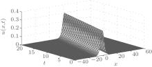
Throughout the simulation the L₂ and L_∞ error norms remain less than 2.3909 × 10^{– 3} and 1.0647 × 10^{– 3} (for d = 1), and 1.3378 × 10^{– 4} and 6.1250 × 10^{– 4} (for d = 0.3). A comparison with the methods in Refs.  [22], [48], [50], [52], [53], [56], and [62] shows that the error norms at times t = 10 and 20, obtained with the present method, are smaller than those obtained with other existing methods (see Table  3). From this Table, it can be seen that the conservation properties (using the exponential spline collocation method) are very good. In comparison with the analytical values for the invariants, for d = 1 and d = 0.3, the relative changes in the invariants are very small. This degree of conservation is superior to that found with the other methods listed in Table 3. The profile of the solitary waves for the MRLW equation with d = 0.3, from time t = 0 to 20, are depicted in Fig.  2.

Fig.  2.

	Figure Option ViewDownloadNew Window
	Fig.  2. Space– time graph of the single solitary wave up to t = 20  s, with d = 0.3, k = 0.01, and h = 0.1, for the MRLW equation, through the interval [0, 100] for x0 = 40.

Table 3.

Table 3.

Table 3. Invariants and errors for single soliton of the MRLW equation for x0 = 40, 0 ≤ x ≤ 100, and different values of d, t, h and k. Methods h k L2 L∞ d = 1, t = 10 0.2 0.025 Analytical 0 0 4.4428829 3.2998316 1.4142135 Our method 2.3909(− 3) 1.0647(− 3) 4.4428827 3.2998042 1.4142107 PGFE[62] 2.4155(− 3) 1.0797(− 3) 4.4431758 3.3003023 1.4146927 PG[22] 3.0053(− 3) 1.6874(− 3) 4.44288 3.29981 1.41416 CBSC-CN[48] 1.639(− 2) 9.24(− 3) 4.442 3.299 1.413 CBSC-PA-CN[48] 2.03(− 2) 1.12(− 2) 4.440 3.296 1.411 CBSC[50] 9.3019(− 3) 5.4371(− 3) 4.44288 3.29983 1.41420 MQ[52] 3.914(− 3) 2.019(− 3) 4.4428829 3.29978 1.414163 d = 1, t = 10 0.1 0.025 Our method 1.9447(− 4) 2.0047(− 4) 4.44249 3.29980 1.41419 QBS[53] 8.644(− 4) 1.2475(− 3) 4.445176 3.302476 1.417411 M1[48] 1.939(− 2) 9.24(− 3) 4.442 9.299 1.413 M3[50] 9.3019(− 3) 5.4371(− 3) 4.44288 3.29983 1.41420 d = 0.3, t = 10 0.2 0.1 Analytical 0 0 3.5819667 1.3450764 0.153723 Our method 1.3378(− 4) 6.1250(− 4) 3.5812102 1.345133 0.1538342 QBS[53] 3.3795(− 4) 7.6729(− 4) 3.582265 1.345182 0.1538901 d = 0.3, t = 20 0.1 0.01 Our method 5.3488(− 5) 3.1778(− 5) 3.5819987 1.3450863 0.1537246 PGFE[62] 8.1125(− 5) 3.5690(− 5) 3.5820204 1.3450974 0.1537250 M3[50] 6.0688(− 4) 2.9665(− 4) 3.58197 1.34508 0.153723 QBS[56] 5.0892(− 5) 2.2228(− 5) 3.581967 1.345076 0.153723 IQ[52] 5.1498(− 5) 2.2551(− 5) 3.5819654 1.3450764 0.153723

Table 3. Invariants and errors for single soliton of the MRLW equation for x0 = 40, 0 ≤ x ≤ 100, and different values of d, t, h and k.

6.1.3. GRLW equation

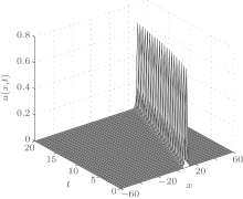
For the purpose of illustration of the presented method for solving the GRLW equation, we consider the case for p ≥ 3 in [− 60, 60] for x₀ = 10. In this test, calculations are carried out with d = 1.01, k = 0.1, h = 0.48, and (p = 4, 6, 8, 10 when the final time is t = 10. Errors in L₂ and L_∞ norms at several times are listed in Table  4 and compared with results in Ref.  [21]. The plot of the estimated solution with d = 0.3 and p = 10, from time t = 0 to 20, are shown in Fig.  3. Throughout the simulation the L₂ and L_∞ error norms remain less than 1.8 × 10^{– 3} and 8.64 × 10^{– 4} for the GRLW equation with different values of p. One can observe from Table  4 that the numerical results calculated with the present method are more accurate in comparison with Ref.  [21].

Table 4.

Table 4.

Table 4. Values of the error norms at different values of t and p for single soliton of the GRLW equation. Methods Error norm t = 2 t = 4 t = 6 t = 8 t = 10 p = 4 Our method L2 2.3(− 5) 4.4(− 5) 6.5(− 5) 8.5(− 5) 1.0(− 4) L∞ 1.6(− 6) 2.7(− 6) 2.5(− 6) 2.6(− 6) 2.4(− 6) Feng et al.[21] L2 1.6(− 4) 3.0(− 4) 4.0(− 4) 4.6(− 4) 5.0(− 4) L∞ 4.0(− 5) 7.0(− 5) 9.0(− 5) 9.0(− 5) 1.0(− 4) p = 6 Our method L2 4.1(− 5) 8.2(− 5) 1.2(− 4) 1.5(− 4) 1.8(− 4) L∞ 1.2(− 5) 2.1(− 5) 2.0(− 5) 2.3(− 5) 2.9(− 5) Feng et al.[21] L2 3.2(− 4) 6.1(− 4) 8.4(− 4) 1.0(− 3) 1.1(− 3) L∞ 1.2(− 4) 2.1(− 4) 2.7(− 4) 3.2(− 4) 3.7(− 4) p = 8 Our method L2 3.8(− 4) 8.1(− 4) 1.2(− 3) 1.5(− 3) 1.8(− 3) L∞ 1.1(− 4) 1.8(− 4) 1.7(− 4) 1.9(− 4) 2.4(− 4) Feng et al.[21] L2 6.3(− 4) 1.1(− 3) 1.6(− 3) 1.9(− 3) 2.2(− 3) L∞ 2.9(− 4) 4.8(− 4) 6.1(− 4) 7.0(− 4) 7.8(− 4) p = 10 Our method L2 8.56(− 4) 1.61(− 3) 1.42(− 3) 1.16(− 3) 1.14(− 3) L∞ 1.02(− 4) 1.70(− 4) 8.64(− 4) 6.31(− 4) 4.61(− 4) Feng et al.[21] L2 1.09(− 3) 1.97(− 3) 2.64(− 3) 3.18(− 3) 3.65(− 3) L∞ 5.5(− 4) 8.5(− 4) 1.07(− 3) 1.23(− 3) 1.36(− 3)

Table 4. Values of the error norms at different values of t and p for single soliton of the GRLW equation.

Fig.  3.

	Figure Option ViewDownloadNew Window
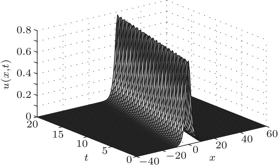
	Fig.  3. Space– time graph of the single solitary wave up to t = 20  s, with d = 1.01, p = 10, k = 0.1, and h = 0.48, for the GRLW equation, through the interval [− 60, 60] for x0 = 10.

6.2. Interaction of two solitary waves

The interaction of two GRLW solitary waves having different amplitudes and traveling in the same direction is illustrated. We consider the GRLW equation with the initial conditions given by the linear sum of two well separated solitary waves of various amplitudes

where

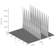
To allow the interaction to occur, the experiment was run from t = 0 to 10 and in the region – 150 ≤ x ≤ 100 for (p = 2, 4, 6, 8 with d₁ = 1.005, d₂ = 1.01, x₁ = 40, x₂ = – 30, h = 0.625, and k = 0.05. Errors in L₂ and L_∞ norms at several times are listed in Table  5 and compared with results in Ref.  [21]. Figure  4 shows the interaction of two soliton solutions of the GRLW equation with p = 8. Throughout the simulation the L₂ and L_∞ error norms remain less than 1.6 × 10^{– 3} and 8.4 × 10^{– 4} for the GRLW equation with different values of p. A comparison with the method used in Ref.  [21] shows that the error norms found with the present method are smaller than those obtained with that method.

Fig.  4.

	Figure Option ViewDownloadNew Window
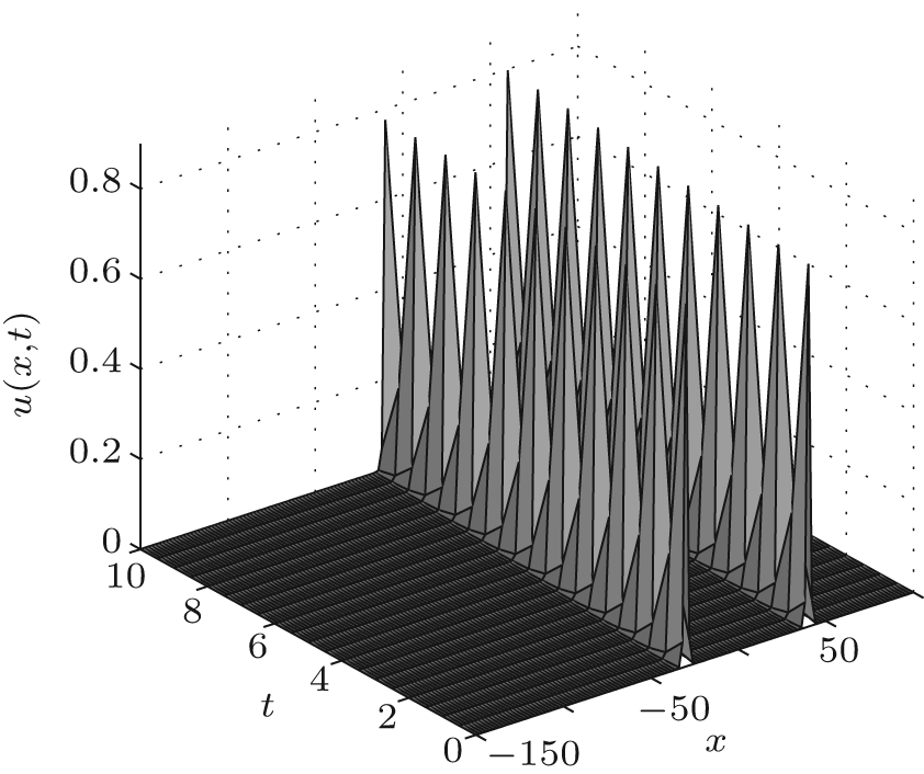	Fig.  4. Space– time graph of the single solitary wave up to t = 10  s, with d1 = 1.005, d2 = 1.01, x1 = 40, x2 = – 30, p = 8, k = 0.05, and h = 0.625, for the GRLW equation, through the interval [− 150, 100].

Table 5.

Table 5.

Table 5. Values of the error norms at different values of t and p for interaction of two solitary solutions of the GRLW equation. Methods Error norm t = 1 t = 2 t = 3 t = 4 t = 5 p = 2 Our method L2 1.6(− 4) 3.0(− 4) 4.0(− 4) 4.7(− 4) 5.1(− 4) L∞ 1.0(− 5) 1.3(− 5) 2.5(− 5) 4.6(− 5) 7.8(− 5) Feng et al.[21] L2 3.3(− 4) 5.1(− 4) 7.0(− 4) 8.6(− 4) 1.0(− 3) L∞ 5.0(− 5) 1.1(− 4) 1.7(− 4) 2.1(− 4) 2.3(− 4) p = 4 Our method L2 1.9(− 4) 3.6(− 4) 5.2(− 4) 6.8(− 4) 8.3(− 4) L∞ 2.0(− 5) 3.3(− 5) 4.0(− 5) 5.3(− 5) 7.4(− 5) Feng et al.[21] L2 8.7(− 4) 1.3(− 3) 1.9(− 3) 2.3(− 3) 2.8(− 3) L∞ 1.2(− 4) 2.7(− 4) 4.1(− 4) 5.2(− 4) 5.6(− 4) p = 6 Our method L2 3.0(− 4) 5.9(− 4) 8.8(− 4) 1.1(− 3) 1.4(− 3) L∞ 2.3(− 5) 3.8(− 5) 4.6(− 5) 5.6(− 5) 8.4(− 4) Feng et al.[21] L2 1.3(− 3) 2.3(− 3) 3.3(− 3) 4.2(− 3) 5.1(− 3) L∞ 3.5(− 4) 6.6(− 4) 9.9(− 4) 1.2(− 3) 1.5(− 3) p = 8 Our method L2 3.2(− 4) 6.5(− 4) 1.0(− 3) 1.3(− 3) 1.6(− 3) L∞ 2.4(− 5) 4.5(− 5) 9.4(− 5) 1.4(− 4) 3.5(− 4) Feng et al.[21] L2 2.0(− 3) 3.8(− 3) 5.5(− 3) 7.2(− 3) 8.9(− 3) L∞ 7.8(− 4) 1.4(− 4) 2.0(− 3) 2.6(− 3) 3.1(− 3)

Table 5. Values of the error norms at different values of t and p for interaction of two solitary solutions of the GRLW equation.

A numerical technique based on a collocation method using exponential B-splines has been presented for the numerical solution of the GRLW equation. The efficiency of the method is tested for the problems of propagation of the single solitary wave, interaction of two solitary waves, and development of an undular bore. The accuracy is examined in terms of the L_∞ and L₂ error norms and the conservation quantities and . Stability analysis is performed by the Von Neumann method and we prove that the new method is unconditionally stable. A convergence analysis for this method is given. The observed errors and invariants are tabulated in Tables and the stability of our presented schemes is verified. These computational results show that our proposed algorithm is effective and accurate in comparison with other existing methods in the literature. The collocation method with exponential B-spline functions provides high accuracy and invariance of the conserved quantities. In addition, the CPU run time of our method is better than for that of the Sinc-collocation method. The superiority of the present method over the previous ones is clear.