The conceptual definitions^[16] of the coordinate system in space are as follows.

The conceptual definitions of coordinate transformation are as follows.

In a right-hand rectangular coordinate system, the rotation matrix that rotates around the X axis in the positive direction can be expressed as

The rotation matrix that rotates around the Y axis in the positive direction can be expressed as

The rotation matrix that rotates around the Z axis in the positive direction can be expressed as

where, θ is the rotation angle. The definition of positive direction is the counterclockwise direction.

The Earth is assumed to be a sphere of uniform density distribution. Then the space target that moves around the Earth can be seen as a particle. The mass concentrates at the center of mass, equivalently. Thus, a simple two-body motion is formed as shown in Fig.  1. Under the two-body motion assumption, the orbit equation is

where h is the relative angular momentum of target per unit mass, i.e., the specific relative angular momentum. Its vector form is is the gravitational constant of the Earth, and its value is 3.986 × 10⁵  km³/s², e ≥ 0 is the eccentricity, and its vector form is . The line defined by the vector e is commonly called the apse line, and f is the true anomaly.

Fig.  1.

	Figure Option ViewDownloadNew Window
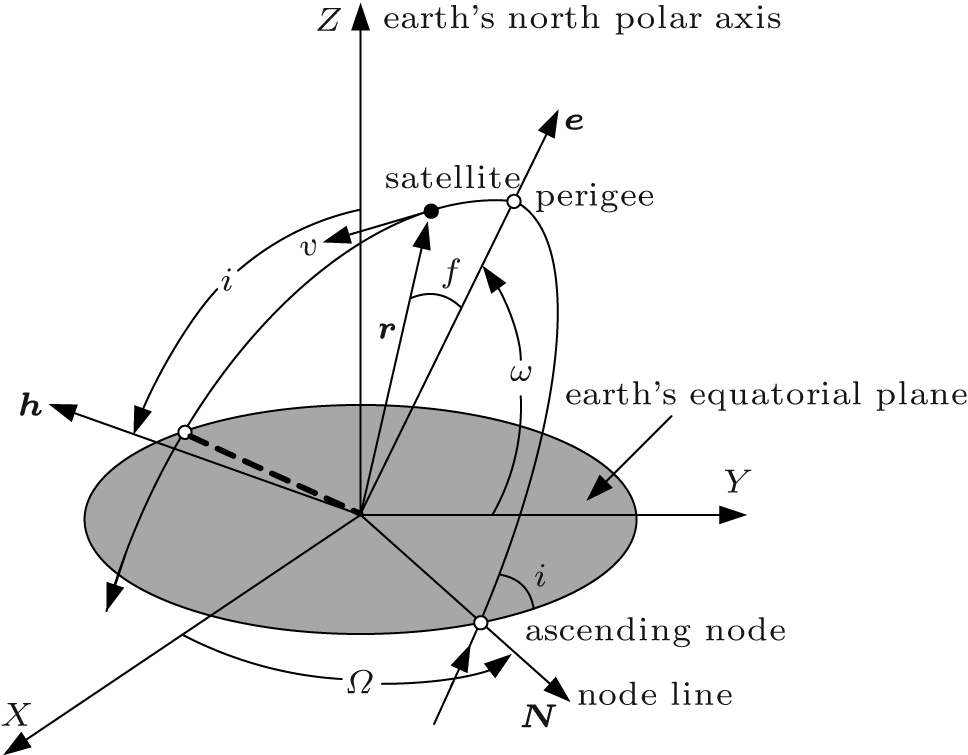	Fig.  1. Satellite orbit model.[17]

Orbit equation  (4) contains three independent parameters: h, e, and f, and it describes the conic sections in the orbital plane. In the actual calculation, the angular momentum h and true anomaly f are frequently replaced by the semi-major axis a and mean anomaly M, respectively. Describing the orientation of an orbit in three dimensions requires three additional parameters, called the Euler angles, which are illustrated in Fig.  1.

First, we locate the intersection of the orbital plane with the equatorial (XY) plane. That line is called the node line. The point on the node line where the orbit passes above the equatorial plane from below it, is called the ascending node. The node line vector N extends outward from the origin through the ascending node. At the other end of the node line, where the orbit dives below the equatorial plane, is the descending node. The angle between the positive X axis and the node line is the first Euler angle Ω , the right ascension of the ascending node. The right ascension is a positive number lying between 0° and 360° .

The dihedral angle between the orbital plane and the equatorial plane is the inclination i, measured according to the right-hand rule, that is, counterclockwise around the node line vector from the equator to the orbit. The inclination is also the angle between the positive Z axis and the normal plane of the orbit. The inclination is a positive number between 0° and 180° .

The third Euler angle ω , the argument of perigee, is the angle between the node line vector N and the eccentricity vector e, measured in the plane of the orbit. The argument of perigee is a positive value between 0° and 360° .

The orbit of the space target can be determined by the six orbital elements (a, M, i, ω , e, Ω ), where the mean anomaly can be expressed as

with E being the eccentric anomaly, and the relationship between the eccentric anomaly and the true anomaly is

Considering the two-body motion, the coordinates of the target’ s center of mass in the geocentric observation coordinate system xyz can be expressed as

where r is the distance from target center to geocentre, and it can be obtained from Eq.  (4).

Assuming that χ _t0 = (a, M_t0, i, ω , e, Ω ) is the target’ s orbital element at the initial observation time, ignoring the influences of precession and nutation on the celestial pole and equinox, the coordinate system xyz can be rotated into coordinate system XYZ by a sequence of three rotations. The first step is to rotate an angle f_t0 + ω around the z axis clockwise. The second step is to rotate an angle i around the x axis clockwise. Finally, we clockwise-rotate around the z axis through an angle Ω . Here, f_t0 is the true anomaly of the initial observation time; it can be obtained by the initial orbital elements through Eqs.  (5) and (6).

Except the mean anomaly, the remaining orbital elements are all constants. The mean anomaly can be obtained by

where t_epoch is the epoch time of initial orbital elements and t₀ is the epoch time of the initial observation time.

At any observation time t, to transfer the coordinate system xyz into XYZ, the only difference relative to initial observation time t₀ is that the rotation angle around the z axis is f_t + ω rather than f_t0 + ω , where f_t is the true anomaly of observation time t.

Therefore, the transformation matrix xyz into XYZ at the observation time t can be written as

where R_x (• ) and R_z (• ) are the rotation matrices around the x axis and z axis, respectively.

Without considering the polar motion, the difference between the geocentric equatorial coordinate system XYZ and the geocentric Earth-fixed coordinate system X′ Y′ Z′ is the Earth’ s rotation angle (i.e., Greenwich hour angle S_G). Then the transformation matrix XYZ into X′ Y′ Z′ can be expressed as

where S_Gt0 is the Greenwich hour angle of the initial observation time t₀, n_E is the Earth’ s rotation angular velocity, and its period is 86164.098903691  s.

The Greenwich hour angle can be calculated from the following equation:

where t_J can be expressed as

with JD(t) being the Julian day at the observation time t, and JD(J2000.0) the Julian day corresponding to epoch J2000.0.

The coordinates of the target in coordinate system X′ Y′ Z′ can be obtained by Eq.  (7) through Eq.  (12) together

Assuming that the longitude, latitude, and elevation of radar are θ _Long, θ _Lat, and h_R, respectively, the radar coordinates in coordinate system X′ Y′ Z′ can be expressed as

where R_E is the radius of the Earth, and generally its value is 6378.15  km.

Using Eqs.  (13) and (14), we can obtain the radar’ s observation vector relative to the target as

For the three-axis-stabilized target, the rotation angular velocity caused by attitude stabilization of the target is equal to the true anomaly, that is, the scatter vector relative to the center of the target is constant in the observation coordinate system. Assuming that the coordinates of some scatter on target are [x_i, y_i, z_i]^T in the geocentric observation coordinate system, the coordinates in the geocentric Earth-fixed coordinate system X′ Y′ Z′ can be written as

where C_α and S_α represent the sine and cosine function of angle α respectively. In the above formula, α = − f_t − ω , β = − i, and γ = − (− S_Gt0 − n_Et + Ω ).

The scatter’ s position vector relative to radar is

From Eq.  (17), we can obtain the distance from radar to the scatter as follows:

We take the first and second derivatives of Eq. (18) to obtain the radial velocity and acceleration:

where ẋ and ẍ respectively represent the first and second derivatives of x, and they can be obtained from Eq.  (17).

Through the orbit simulation based on the two-body model, we can obtain the position of the target from Eq.  (16) and also obtain the radar position from Eq.  (14) in the geocentric Earth-fixed coordinate system X′ Y′ Z′ at any time. Bistatic ISAR consists of two radars placed at different places, and the scatter’ s position vector and other parameters (radial velocity, acceleration, and so on) relative to either radar can be obtained.

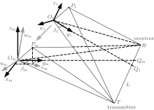
Figure  2 illustrates the topology of bistatic ISAR imaging plane, where oxyz is the right-hand coordinate system with its origin o located at the target’ s center, and the x axis points to the transmitter. The y axis lying in the bistatic plane is perpendicular to the x axis. The z axis forms a right-hand rectangular coordinate system with the x axis and y axis. and denote the target’ s line of sight (LOS) unit vectors pointing to the transmitter and receiver respectively. The target rotates around o, and its effective rotation vector is ω _Σ .

Fig.  2.

	Figure Option ViewDownloadNew Window
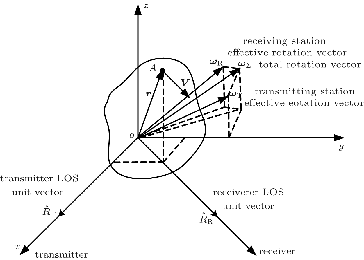	Fig.  2. General topology of bistatic ISAR imaging plane.

For some scatter A on the target, its position vector is r, then the velocity V of scatter A caused by target rotation can be expressed as

Note that the bistatic Doppler frequency is the summation of the Doppler frequency created by the velocity vector respectively on the transmitter LOS and receiver LOS. Then the instantaneous rotation bistatic Doppler frequency of scatter A could be given as

Substituting Eq.  (21) into Eq.  (22) leads to

Let ω _T represent the projection vector of ω _Σ on the plane perpendicular to , and ω _R denotes the projection vector of ω _Σ on the plane perpendicular to , then we will have

Substituting Eq.  (24) into Eq.  (23) yields

We can see that the bistatic Doppler frequency is the projection of position vector r on vector , that is, is the cross range direction. As is well known, the range direction is the gradient vector of an equidistant surface. Since the equidistant surface of bistatic radar is of an ellipse whose foci are at the transmitter and receiver respectively, its gradient vector direction is the direction of bistatic angle bisector, i.e., the direction of vector .

Thus, the range direction of bistatic ISAR is determined by

and the cross range direction of bistatic ISAR is determined by

Vectors Θ and 𝚵 determine the imaging plane, and the signs of vectors Θ and 𝚵 have no effect on the imaging plane determination. We can also see that the vector Θ is always perpendicular to 𝚵 in the case of the turntable model.

The motion forms of the space three-axis-stabilized target include the translational motion and the rotation around the target center of mass. The translational motion of the target will cause the change of visual angle, which can also provide the bistatic Doppler frequency. Thus, the cross range direction is determined by both the translational motion and the rotation.

Assume that the translational motion velocity is υ . Note that υ here is different from the rotation velocity V. We know that the radial velocity relative to transmitter and receiver cannot cause the visual angle to change. Let v_T represent the projection vector of v on the plane perpendicular to , and υ _R denote the projection vector of υ on the plane perpendicular to , then we will have

Then the total rotation vector consists of two parts, one is caused by the translational motion and the other by attitude-stabilized rotation. Let ω _vT and ω _vR be the rotation vectors caused by translational motion relative to transmitter and receiver respectively, then they will be expressed respectively as

where R_T and R_R are the distances from the center of target to transmitter and to receiver, respectively. Assuming that the attitude-stabilized rotation vector is ω _s, and ω _sT is the projection of ω _s on the plane perpendicular to is the projection of ω _s on the plane perpendicular to , then

The total rotation vectors ω _{∑ T} and ω _{∑ R} of the target relative to transmitter and receiver can be written as

Substituting Eqs.  (29)– (31) into Eq.  (27), we obtain the cross range direction of bistatic ISAR of three-axis-stabilized target.

According to vector product formula a × b × c = (a · c) b − (b · c) a, we can obtain that

Substituting Eqs.  (33) and (34) into Eq.  (32) yields

Let

and

then 𝚵 ₁ which is similar to Eq.  (27) will be a cross range vector caused by attitude-stabilized rotation, and 𝚵 ₂ is the cross range vector caused by the translational motion of target.

The bistatic ISAR range direction of the three-axis-stabilized target is also the direction of bistatic angle bisector, and it can be written as

Note that the vector Θ is not always perpendicular to vector 𝚵 .

The space target can be regarded as the cooperative target, and we can obtain its position vector and velocity vector at any time through the six orbital elements. Then the cross range direction 𝚵 and range direction Θ can be obtained according to Eqs.  (35) and (36). Θ and 𝚵 together determine the imaging plane.

When the imaging plane is spatial-variant, the geometry of bistatic ISAR is shown in Fig.  3, where T is the transmitter, R is the receiver, and L denotes the length of the baseline of bistatic ISAR. At the imaging initial time t₁, a right-hand coordinate system x₁y₁z₁ is established. Its origin O₁ is at the center of the target, the y₁ axis is the range axis, i.e., the bistatic angle bisector direction. The x₁ axis is perpendicular to the y₁ axis in the bistatic plane, and the z₁ axis is perpendicular to the x₁O₁y₁ plane. P is a scatter on the target, at the time t₁, we denote it as P₁, and its coordinates are (x_P, y_P, z_p) in the x₁y₁z₁ system. At the imaging time t_m, O_m is the center of the target and we write the scatter P as P_m. Based on this, a right-hand coordinate system x_my_mz_m is established with O_m representing its origin, the y_m axis pointing to the bistatic angle bisector direction, the x_m axis being perpendicular to the y_m axis in the bistatic plane, and the z_m axis perpendicular to the x_mO_my_m plane. In the coordinate system x_my_mz_m, the coordinates of scatter P_m are (x_Pm, y_Pm, z_pm). At the times t₁ and t_m, the bistatic angles are β ₁ and β _m, and the intersections of the bistatic angle bisector with the baseline are Q₁ and Q_m, respectively.

Fig.  3.

	Figure Option ViewDownloadNew Window
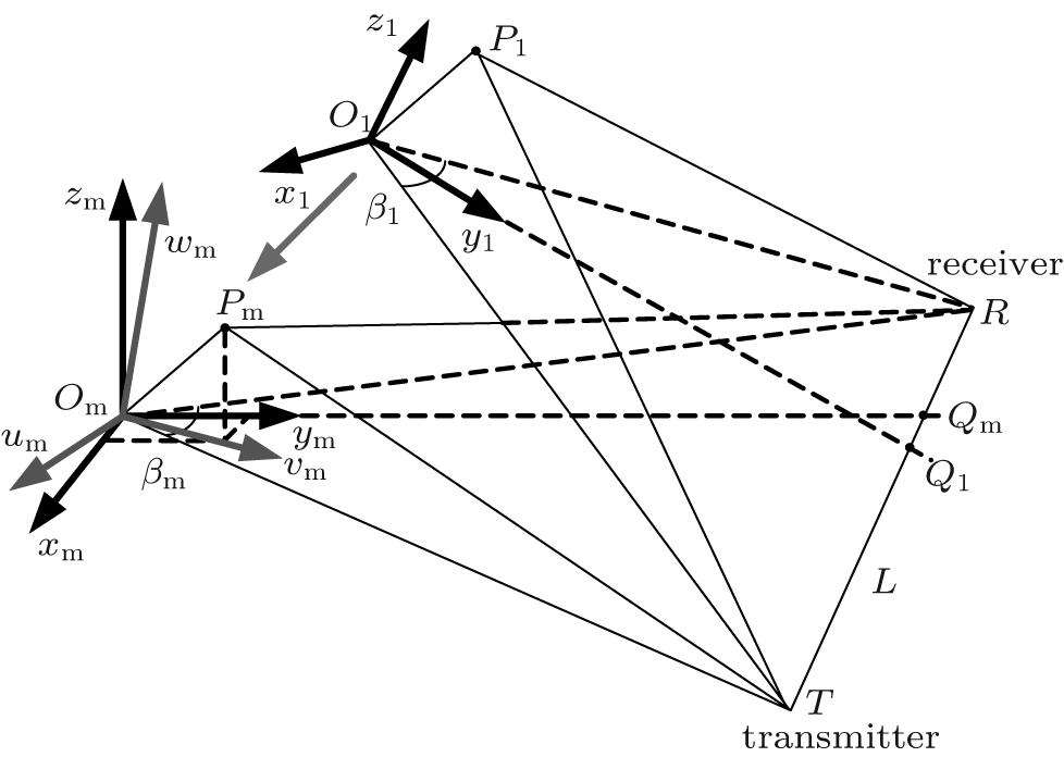	Fig.  3. Geometry of bistatic ISAR.

The space three-axis-stabilized target also rotates while it has the translational motion component. The rotation causes the change of the scatter projection position as well as the translational motion. The rotation axis goes through the center of the target and it is parallel to the normal line of the orbital plane. During imaging, the rotation axis and rotation angular velocity can be regarded as constants. The process that the target rotates around the rotation axis is equivalent to that the target stays stationary (i.e., translational motion only) and the radars rotate around the rotation axis inversely along with the coordinate system. After the rotation of radars and the coordinate system, a new coordinate system is obtained. The scatters’ coordinate values in the new coordinate system reflect not only the different look angles but also the target’ s attitude-stabilized rotation. From the coordinate values we can obtain the range histories of any scatter, and the Doppler frequency can be easily found by taking the slow time derivative of range histories.

Assuming that the attitude-stabilized rotation unit vector of the target is A(A_x, A_y, A_z). From t₁ to t_m, the rotation angle is − η _m. Note that the minus sign represents the clockwise rotation. Then counterclockwise rotating the space coordinate system x_my_mz_m around rotation axis A through the angle η _m, we can obtain a new coordinate system u_mv_mw_m, and it implies the attitude-stabilized rotation of the target. Let be the three axis unit vectors of coordinate system be the three axis unit vectors of coordinate system be the three axis unit vectors of coordinate system u_mv_mw_m. All the unit vectors are row vectors of 1 × 3 in size. Since u_mv_mw_m is obtained from x_my_mz_m, according to Eqs.  (A18) and (A19) in Appendix A, we can obtain that

The transformation matrix R_s(η _m) is derived in Appendix A.

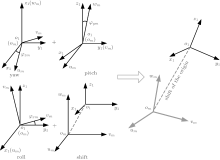
Since the coordinates of scatter P₁ are (x_p, y_p, z_p) in the x₁y₁z₁ system, to obtain the coordinates of P_m in u_mv_mw_m, it is necessary to deduce the transformation relationship between x₁y₁z₁ and u_mv_mw_m. As is well known, any two rectangular coordinate systems in space can be mutually transformed by a sequence of three rotations and a shift of the origin, which is illustrated in Fig.  4. Three rotations are the Euler angles, i.e., yaw angle, pitch angle, and roll angle. We define that the yaw angle is the angle rotating around the z axis, the pitch angle is the angle rotating around the y axis, and the roll angle is the angle rotating around the x axis. The shift of the origin has no influence on the directions of coordinate axes. Without considering the origin position, to transfer the x₁y₁z₁ system into the u_mv_mw_m system, we need three rotations.

The first step is to rotate the x₁o₁y₁ through a yaw angle φ _zm around the z₁ axis. Then we obtain a new coordinate system , and the directions of the axis are the same. We can obtain the orthogonal transformation matrix R_z (φ _zm) by Eq.  (3).

The second step is to rotate the through a pitch angle φ _ym around the axis. Then we obtain a new coordinate system , and the directions of the axis and axis are the same. We can obtain the orthogonal transformation matrix R_y (φ _ym) by Eq.  (2).

The third step, i.e., the last step is to rotate the through a roll angle φ _xm around the axis. Then we obtain a new coordinate system , and the directions of the axis and axis are the same. We can obtain the orthogonal transformation matrix R_x (φ _xm) by Eq.  (1).

Fig.  4.

	Figure Option ViewDownloadNew Window
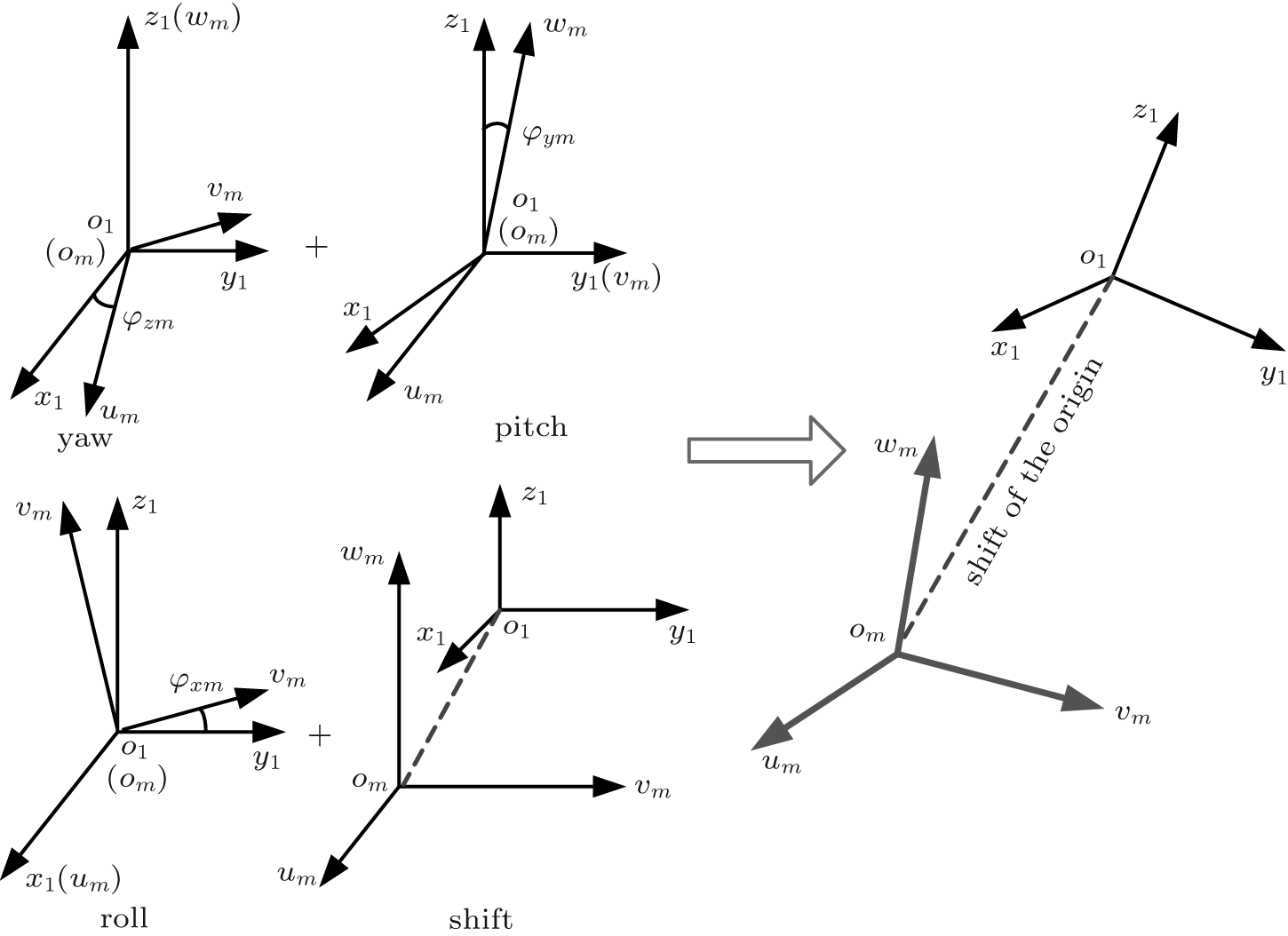	Fig.  4. Schematic diagram of coordinate transformation in space.

There always exists a set of Euler angles φ _zm, φ _ym, and φ _xm so that the directions of and u_mv_mw_m are totally the same. Let ξ _zm, ξ _ym and ξ _xm be the Euler angles satisfying this condition. Then the transformation matrix transferring the x₁y₁z₁ system into the u_mv_mw_m system is the product of the three matrices obtained above, i.e.,

Then the axial directions of u_mv_mw_m and x₁y₁z₁ satisfy the following equation:

The transformation matrix R_{xyz_m} can be expressed as

Since the axial directions of x₁y₁z₁ and x_my_mz_m can be determined by Eqs.  (35) and (36), and the axial directions of u_mv_mw_m can be obtained by Eq.  (37) further, we can obtain the transformation matrix R_{xyz_m} by Eq.  (40). By combining Eqs.  (38) and (40), we obtain the solutions of the three Euler angles as follows:

In theory, the limits of Euler angles are [− π , π ]. The yaw angle ξ _zm is the rotation angle around the normal line to the imaging plane, and essentially it is the integration angle used to obtain the required cross range resolution. The pitch angle ξ _ym and roll angle ξ _xm are the rotation angles around the range axis and cross range axis respectively, and they are the spatial-variant angles that reflect the spatial-variant properties of the imaging plane. As is well known, when the integration rotation angle is big, the migration through the resolution cell may occur in the bistatic ISAR, which will affect the imaging quality. So in actual imaging, to ensure the imaging quality, the integration rotation angle is generally not more than 6° ∼ 7° . Thus, in the general case, the Euler angles are small, and the limit [− π /18, π /18] is sufficient to meet the need. Note that the limit has no effect on the subsequent data processing.

The coordinates of scatter P₁ are (x_p, y_p, z_p) in the x₁y₁z₁ system, and the coordinates of scatter P_m are (u_pm, v_pm, w_pm) in the u_mv_mw_m system, which satisfy the following equation.:

Combining Eqs.  (39) and (44), we can obtain the coordinates of scatter P_m as

Since R_{xyz_m} is a unit orthogonal matrix, the inverse of R_{xyz_m} is its transpose matrix, i.e. . Equation  (45) can be rewritten as

By using Eq.  (46), we can obtain the position histories of scatter P projected onto the imaging plane during imaging.

Assuming that the two radars are ideally synchronous, and the transmitter emits a chirp signal with a period of T_PRT, we have

where rect (u) is the rectangular window function defined as (u) = 1 if |u| ≤ 0.5 and (u) = 0 otherwise; is the fast time; t_m = mT_PRT, (m = 0, 1, 2, … ) is the transmitting time, named slow time; t is the total time and T_p is the pulse width; f_c is the carrier frequency; μ is the chirp rate.

At the time t_m, let Δ R_pm be the difference between the sum of the distance from scatter P_m to two radars (transmitter and receiver) and the sum of the distance from the center of the target to two radars. We can obtain the range profile of scatter P_m through pulse compression. Then the range profile after ideal motion compensation can be written as^{[8, 18]}

where A_p is the signal amplitude, and c is the speed of light in free space. From Eq.  (48), the peak position of the range profile occurs at the time . The Doppler frequency can be expressed as

obtained from the phase.

In bistatic ISAR, the length of Δ R_pm is 2 cos(β _m/2) times the length of the projection of vector O_mP_m onto the bistatic angle bisector, ^[19] that is, the value of R_pm is 2 cos (β _m/2) times the coordinate value of scatter P_m onto the range axis in the u_mv_mw_m system. Taking the attitude-stabilized rotation into account, the range axis is the v_m axis, and then the range projection value v_pm of scatter P_m onto the range axis can be obtained by Eqs.  (38) and (46) as follows:

We can write R_pm as

Using Eq.  (50), the instantaneous frequency of scatter P_m can be found by taking the slow derivative of the phase in Eq.  (48) as follows:

where ξ ′ = dξ /dt_m represents the derivative of the slow time. Equations  (50) and (51) describe the range histories and Doppler histories during imaging, respectively. When the values of yaw angle ξ _zm, pitch angle ξ _ym, roll angle ξ _xm, and bistatic angle β _m change, the peak positions of range and Doppler frequency also change; it may cause the migration through resolution cells, which may result in image blurring. Thus equations  (50) and (51) are the evidences of image quality analysis. For different imaging segments, the Euler angles and bistatic angle have different variation characteristics, and the degrees of migration through resolution cells differ from each other. Then we obtain different quality ISAR images further. So it is necessary to analyze the influence of each angle on image quality, which provides a theoretical guidance for imaging experiment and the selection of imaging segments.

The above two equations are quite complex, especially Eq.  (51). Considering that the yaw angle, pitch angle, and roll angle are all very small, the cosine term can be replaced by 1, and their high order sine terms (order greater than or equal to 3) can be ignored. Then equations  (50) and (51) can be simplified into

Both equations can be written as the superposition of non-spatial-variant terms and spatial-variant additional terms, i.e.,

where

where Δ R_{pm_z} and f_{d_z} are the range information and Doppler information of scatter when the imaging plane has no spatial-variant property, and R_{pm_xy} and f_{d_xy} are the range terms and Doppler terms caused by the spatial-variant imaging plane. When analyzing the effect of the spatial-variant property on imaging, we only need to analyze Eqs.  (57) and (59).

The spatial-variant property of bistatic ISAR is concerned with the target motion trajectory and the positions of transmitter and receiver. When the spatial-variant property is serious, the phenomenon of migration through resolution cells occurs, which may result in image blurring. The analysis of the spatial-variant property provides evidence for imaging experiment and the selection of imaging segments.

We select the Tiangong-1 satellite as the simulation target, and its six orbital elements are provided by the Space Surveillance Network (SSN) of America in the form of a two-line element (TLE) listed as follows:

1 37820U 11053A 14104.86088755 0.00057267 00000-0 50311-3 0 9357

2 37820 042.7734 335.3498 0012276 284.0961 185.9363 15.67862963146089

The epoch time of initial orbital elements is on 14 April 2014 at 20:39:41. The six orbital elements can be derived from the TLE. Then we can simulate the motion of a satellite in orbit according to the model built in Section  2. Placing the transmitting station in city A, and placing the receiving station in city B, from 05:39:30 to 05:47:50, i.e., in a total time of 500 s the satellite was visible by using the transmitter and receiver. The simulation scenario is shown in Fig.  5, where the solid curve represents the satellite orbit, the diamond denotes a transmitter and the circle refers to a receiver, and the star is the geocentric position. The coordinate system is the Earth-fixed system.

Fig.  5.

	Figure Option ViewDownloadNew Window
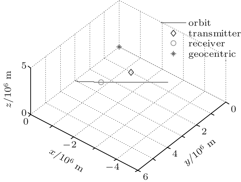	Fig.  5. Simulation scenario.

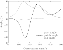
To describe the spatial-variant property of the imaging plane intuitively, we simulate the yaw angle, pitch angle, and roll angle curves in steps of 10  s, the results of which are shown in Fig.  6. In the figure, the yaw angle (i.e., integration angle) and pitch angle change greatly but the roll angle has a small variation.

Fig.  6.

	Figure Option ViewDownloadNew Window
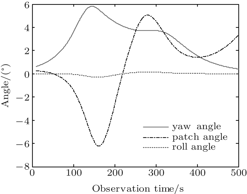	Fig.  6. Spatial-variant angle curves every 10  s.

The purpose of spatial-variant analysis is to analyze the effect of a changing imaging plane on image quality. The range terms and Doppler terms caused by the spatial-variant imaging plane are shown in Eqs.  (57) and (59), where range terms Δ R_{pm_xy} contain two factors and Doppler terms f_{d_xy} contain five factors. These seven factors can be written as follows:

Range factor 1,

Range factor 2,

Doppler factor 1,

Doppler factor 2,

Doppler factor 3,

Doppler factor 4,

Doppler factor 5,

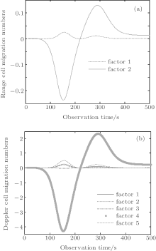
These factors reflect the degree of migration through range and Doppler cells. Let the size of target be 10  m, i.e., x_p = y_p = z_p = 10  m, then we will simulate the possible numbers of migration through the range and Doppler cell by the above seven factors also in steps of 10  s. The results are shown in Fig.  7. Figure  7(a) shows the variations of the number of range cell migrations with observation time, and figure  7(b) displays variations of the number of Doppler cell migrations with observation time. We can see that the migration through range cell number is less than 0.25 for a target of this size. However, the Doppler cell number that the migration goes through is greater than 4 at some orbital segments. In addition, it is caused mainly by Doppler factor 4. Doppler factor 4 is a function of the roll angle and height coordinate of scatter. If the scatter has the larger height coordinate, more serious Doppler cell migrations will take place. Therefore, for some imaging segments, the spatial-variant property will deteriorate the image quality. Since the existing correction algorithm^[20] cannot correct the Doppler migration caused by the spatial-variant imaging plane, to obtain a high-quality ISAR image, we need to avoid the orbital segments which have a serious spatial-variant property in actual imaging.

Fig.  7.

	Figure Option ViewDownloadNew Window
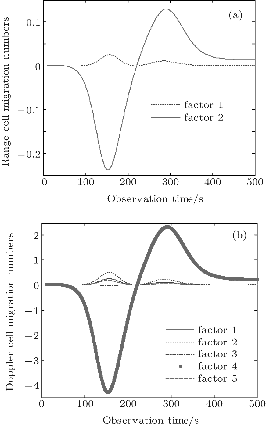	Fig.  7. The numbers of migrations through range and Doppler cell caused by spatial-variant imaging plane versus observation time: (a) range cell migration numbers; (b) Doppler cell migration numbers.

From the above simulation, we can see that the spatial-variant property has little effect on migration through range cell, but has great Doppler migration. To verify the above analysis, the imaging simulations are carried out.

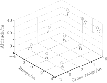
Two different imaging segments are selected for the bistatic ISAR imaging simulation. The observation time for imaging segment 1 is from 145  s to 155  s. The spatial-variant property is serious and it will cause the great image change of different height scatters in theory. The observation time for imaging segment 2 is from 215  s to 225  s. The imaging plane is quite stable with respect to segment 1, and the imaging results of discrete scatters at different heights should be basically the same. The simulation scatter model is shown in Fig.  8, and the coordinate values of 9 scatters are listed in Table  1. The values of range and cross range are as small as 3  m, but the height difference is large, the height coordinate values of scatters A ∼ C are 0  m, scatters D ∼ F are 15  m, and scatters G ∼ I are 30  m. The simulation radar parameters and imaging parameters of two imaging segments are listed in Table  2.

Fig.  8.

	Figure Option ViewDownloadNew Window
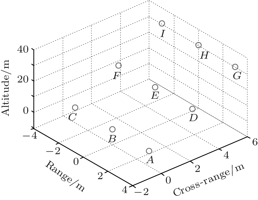	Fig.  8. Scatter model.

Table 1.

Table 1.

Table 1. Coordinate values of scatters. A B C D E F G H I Range/m 3 0 – 3 3 0 – 3 3 0 – 3 Cross-range/m 0 0 0 3 3 3 6 6 6 Altitude/m 0 0 0 15 15 15 30 30 30

Table 1. Coordinate values of scatters.

Table 2.

Table 2.

Table 2. Simulation radar parameters and imaging parameters of bistatic ISAR. Parameter name Parameter value Parameter name Parameter value Parameter name Parameter value Imaging segment 1 Imaging segment 2 Carrier frequency 10  GHz PRF 50  Hz mean bistatic angle 90.78° 114.03° Bandwidth 1  GHz integration pulses 500 integration rotation angle 5.68° 4.02° Pulse width 20  μ ms integration time 10 s range resolution 0.214  m 0.276  m Sampling rate 1.25  GHz imaging algorithm RD coherent imaging cross range resolution 0.215  m 0.393  m

Table 2. Simulation radar parameters and imaging parameters of bistatic ISAR.

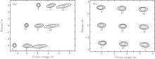
The imaging results are shown in Fig.  9. As we can see in Fig.  9(a), the difference of imaging results is quite significant for different height scatters: the higher the scatters, the worse the imaging results are. The scatters in Fig.  9(b) have the same qualities. The reason for the difference between the two figures is that the spatial-variant property is serious in segment 1, which results in migration through Doppler cells of the higher scatters. Note that the image in Fig.  9(a) is askew with respect to the scatter model, which is the image distortion caused by the time-varying bistatic angle.^[15]

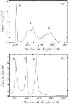
To quantitatively analyze the effect of height on migration through Doppler cells, the range cell where scatters B, E, and H stay, is extracted. The cross range results of two imaging segments are shown in Fig.  10. The difference in amplitude among the three scatters is large in segment 1, and the scatters E and H have serious mainlobe expansion. The scatters in segment 2 change a little.

Fig.  9.

	Figure Option ViewDownloadNew Window
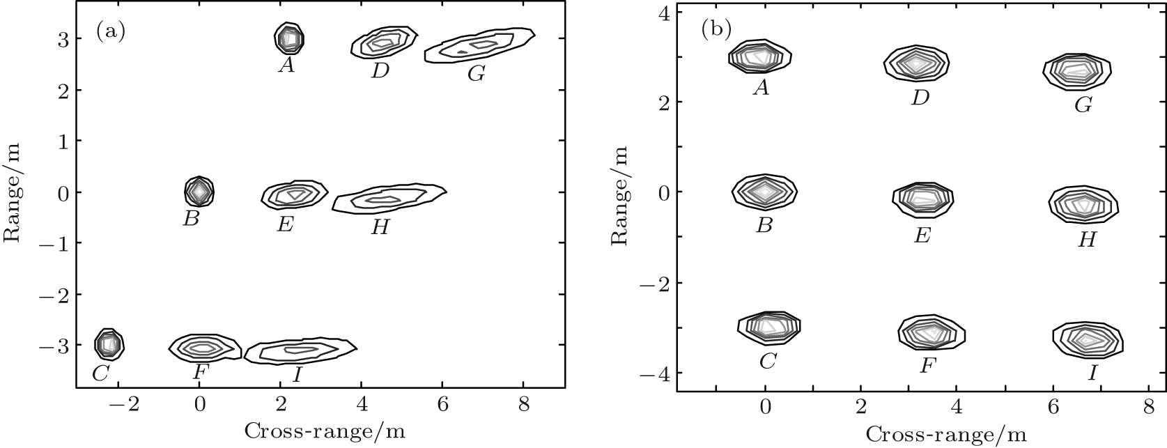	Fig.  9. Imaging results of two segments: (a) segment 1; (b) segment 2.

We calculate the range and cross range 3-dB mainlobe widths of scatters at different heights of the two imaging segments, and list the results in Table  3. In segment 1, the range 3-dB mainlobe widths of different scatters changes a little, but the cross range 3-dB mainlobe width occupies 1, 6, and 12 cross range cells when the heights are 0, 15, and 30  m. Compared with the result in Fig.  7(b), the scatter at the height of 30  m will cause about 12 Doppler cells to migrate, the imaging results of bistatic ISAR perfectly match the results in Fig.  7(b). The above results indicate the correctness of the analysis of the spatial-variant property. In segment 2, the range and cross range 3-dB mainlobe widths of different scatters are nearly the same. The results also confirm the conclusion shown in Fig.  7.

Table 3.

Table 3.

Table 3. Statistical results of 3-dB mainlobe width. 3-dB mainlobe width of range bin/m 3-dB mainlobe width of cross-range bin/m Segment 1 Segment 2 Segment 1 Segment 2 Altitude 0  m (A, B, C) 0.219 0.285  m 0.220 0.405 Altitude 15  m (D, E, F) 0.239 0.285  m 1.257 0.417 Altitude 30  m (G, H, I) 0.252 0.287  m 2.553 0.417

Table 3. Statistical results of 3-dB mainlobe width.

From the comparison between spatial-variant angle and bistatic ISAR imaging results, the actual imaging results are quite consistent with the theoretical analysis, which shows the correctness of the research on the spatial-variant property.

Fig.  10.

	Figure Option ViewDownloadNew Window
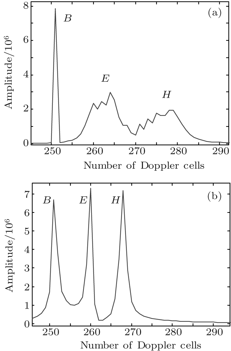	Fig.  10. Comparisons of cross section between scatters at different heights: (a) segment 1 and (b) segment 2.