As this research primarily aims to model the driving behaviors induced by the traffic signal, a one-dimensional lattice is adopted to construct a single lane road segment with a traffic light which is operated in a fixed cycle manner. As shown in Fig. 1, the road segment consists of three sections, i.e., A, B, and C. Section A represents the part on which the vehicles are not affected by the traffic light, possibly due to the low visibility. The effective point is where the vehicular movement begins to be affected by the traffic signal operation. Sections B and C are separated by the traffic light, as different driving behaviors typically manifest in reality for the sections before and after a traffic light. All road sections are subdivided into a number of cells with the same length. Each cell is either empty or occupied by one vehicle travelling with a discrete velocity ranging from v_min to v_max. In this paper, it is assumed that the maximum permitted velocity v_max is the same for all sections. For simplicity, one type of vehicle and homogeneous driver are assumed in the following.

Fig. 1.

	Figure Option ViewDownloadNew Window
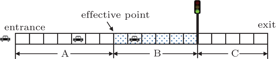	Fig. 1. The signal controlled traffic scenario.

To realize the dynamics for different road sections, the proposed model consists of two sets of rules, one for the normal sections (i.e., sections A and C) where only the reaction to the preceding vehicle exists and the other for the effective section (i.e., section B) where the vehicular movement is affected by both the preceding vehicle and the traffic signal.

Before explaining the rules, the definitions on the variables and parameters used in the model are given as follows. Let T_g, T_r, and T_y be the lengths of green, red and yellow phases, respectively, and t̄ _g, t̄ _r, and t̄ _y be the remaining time for each phase. τ _i is the amount of time for which the vehicle i has been stopped. Let x_i and v_i denote the position and velocity, respectively, of vehicle i, and x_{i− 1} and v_{i− 1} be the position and velocity, respectively, of the vehicle ahead. a_max and b_max denote the maximum acceleration and deceleration per time step. In this paper, the vehicle is allowed to accelerate at a rate from 1 to a_max or decelerate at a rate from 1 to b_max. Note that only an integer is allowed for the rates. Thus, the number of candidate acceleration rates n_a and the number of candidate deceleration rates n_b are equal to a_max and b_max, respectively. While g_i denotes the gap from the vehicle to its predecessor, G_i is the distance from its current location to the stop line (i.e., the same position as the traffic light in this paper). p_gm, p_gs, p_ym, p_ys, p_rm1, and p_rs, denote the probabilities to be taken for the random deceleration for the moving and stopped vehicles during green, yellow, and red phases, respectively.

As the proposed model adopts limited acceleration and deceleration capabilities for vehicles, a full speed or a complete stop may require more than one time step of acceleration or deceleration. Thus, in order to determine the safe distances from the vehicle to its predecessor and the traffic light, two distances, and , are defined as

where

The distance between two successive vehicles estimated in Eq. (1) takes into account the worst situation where the leading vehicle i − 1 continually brakes at the maximum rate until it stops and the corresponding distance is defined as d_{leadi− 1} (t). The distance d_{leadi− 1} (t) together with the gap g_i (t) is the total distance that vehicle i can travel before collision to the leading vehicle in the worst situation. is the distance when vehicle i attempts to change its velocity at the rate of δ _k (δ _k∈ {− b_max, … , − 1, 0, 1, … , a_max) at time step t + 1 and then decelerate at the rate of b_max at the subsequent time steps until it stops. M_{i− 1} = ⌊ v_{i− 1}(t)/b_max⌋ (⌊ ⌋ denotes the floor function) is the number of time steps required by vehicle i − 1 to come to a stop after a sequence of decelerations. On the other hand, the time steps required by vehicle i to come to a stop from v_i(t) + δ _k can be estimated by N_i = ⌊ (v_i(t) + δ _k)/b_max⌋ . Similarly, in Eq. (2) denotes the remaining distance between the traffic light and the vehicle after it firstly alters its velocity at δ _k and then decelerates to zero at the maximum rate. Note that a non-negative value of or indicates that the vehicle can travel with the desired velocity without traffic collision or violation and therefore the corresponding distance is called the safe distance in this paper.

1) Rules for the effective section Table 1 briefly summarizes the driving behaviors typically observed in reality for the vehicles approaching a traffic light and corresponding rules developed for the velocity update.

Table 1.

Table 1.

Table 1. Typical driving behaviors and the corresponding velocity update rules for the vehicles on the effective section. Phase Moving vehicles (vi(t) > 0) Stopped vehicles (vi(t) = 0) Green Fast movement Slow-to-start at the beginning R1: Obtain based on Eq. (1) with − bmax ≤ δ k ≤ amax; R2: vi(t + 1/2) → max(min(vi(t) + δ vehi(t), vmax), 0), where δ vehi is the velocity increment that results in the minimum distance in P; R3: vi(t + 1) → max{vi(t + 1/2)− 1, vi(t)− bmax, 0} with pgm. R1: Obtain based on Eq. (1) with 0 ≤ δ k ≤ amax; R2: vi(t + 1/2) → max(min(vi(t) + δ vehi(t), vmax), 0), where δ vehi is the velocity increment that results in the minimum distance in P; R3: vi(t + 1) → max{vi(t + 1/2) − amax, 0} with pgs = min{pmax, pgm + 0.01τ i}. Yellow Slow-down if it cannot pass Inch-forward to reduce the gap R1: Obtain and based on Eqs. (1) and (2) with − bmax ≤ δ k ≤ amax if Gi(t)/vi(t) < t̄ y or − bmax ≤ δ k ≤ 0 if Gi(t)/vi(t) ≥ t̄ y; R2: vi(t + 1/2) → max(min(vi(t) + δ vehi(t), vmax), 0) if Gi(t)/vi(t) < t̄ y or vi(t + 1/2) → max(min(vi(t) + δ vehi(t), vi(t) + δ lighti(t), vmax), 0) if Gi(t)/vi(t) ≥ t̄ y (where δ vehi and δ lighti are the velocity increments that result in the minimum distances in P and Q); R3: vi(t + 1) → max{vi(t + 1/2) − 1, vi(t) − bmax, 0} with pym if Gi(t)/vi(t) ≥ t̄ y. R1: Obtain and based on Eqs. (1) and (2) with 0 ≤ δ k ≤ 1; R2: vi(t + 1/2) → max(min(vi(t) + δ vehi(t), vi(t) + δ lighti(t), vmax), 0) (where δ vehi and δ lighti are the velocity increments that result in the minimum distances in P and Q); R3: vi(t + 1) → max{vi(t + 1/2) − 1, 0} with pys. Red Slow-down in advance Inch-forward to reduce the gap R1: Obtain and based on Eqs. (1) and (2) with − bmax ≤ δ k ≤ 0; R2: vi(t + 1/2) → max(min(vi(t) + δ vehi(t), vi(t) + δ lighti(t), vmax), 0) (where δ vehi and δ lighti are the velocity increments that result in the minimum distances in P and Q); R3: if vi(t + 1/2) > 0, vi(t + 1) → max{vi(t + 1/2) − 1, vi(t) − bmax, vmin} where vmin = 1 with prm1 and vmin = 0 with prm0. R1: Obtain and based on Eqs. (1) and (2) with 0 ≤ δ k ≤ 1; R2: vi(t + 1/2) → max(min(vi(t) + δ vehi(t), vi(t) + δ lighti(t), vmax), 0) (where δ vehi and δ lighti are the velocity increments that result in the minimum distances in P and Q); R3: vi(t + 1) → max{vi(t + 1/2) − 1, 0} with prs.

Table 1. Typical driving behaviors and the corresponding velocity update rules for the vehicles on the effective section.

For the green phase, three rules have been designed for the velocity update so as to reflect the fast movement for the moving vehicles. First of all, the set of safe distances P is calculated according to Eq. (1) for δ _k ranging from − b_max to a_max. Then, the velocity increment δ _vehi that results in a minimum safe distance will be selected. This implies the intention of drivers to cross an intersection as fast as possible, provided the movement is safe. In addition, it has been found that many drivers decelerate without any exogenous reasons on the highway.^[1] This may not be common for the signalized traffic, as more drivers would concentrate on driving when approaching an intersection where there are likely to be more traffic conflicts. Thus, a small probability should be assigned to the random deceleration (i.e., R3). Note that only a small deceleration rate (i.e., 1 cell/step²) is allowed in R3 to reflect the fast movement.

It is quite common that drivers stop focussing their attention on the signal while waiting at signalized intersections and may initiate other activities (e.g., making a call, playing with their mobile phone, reading newspapers, cleaning up windows, etc.), potentially resulting in a slow-to-start^{[7, 21, 22]} when the light changes to green. Thus, this slow reaction is a typical behavior that the proposed model attempts to incorporate for a stopped vehicle. The first two rules are the same as those for the moving vehicles during green phase, except that only acceleration is allowed for the stopped vehicle (i.e., 0 ≤ δ _k ≤ a_max). However, the stopped vehicles may still be motionless with probability p_gs (in R3), which is dependent on the stopped time. We have adopted a linear increasing function of the stopped time as that in Ref. [12]. The probability p_gs should be larger than p_gm, as a stopped vehicle generally takes more time to start than a moving one due to the inertia of the vehicle or the reaction delay.^[21]

A simple mechanism has been designed to govern the vehicular motion during the yellow light. That is, a vehicle will move forward, if it can pass the traffic light location at the current velocity before the termination of the yellow light, and come to a stop, otherwise. Note that this mechanism implies an assumption that drivers know exactly the remaining time of yellow light. Such an assumption is not true in reality and the incomplete knowledge of yellow time often means that drivers are in a dilemma potentially resulting in red-running. However, the model proposed in this paper endeavors to avoid any traffic violations and this explains why such an unrealistic assumption is made in the model. The first rule is used to obtain two sets of safe distances P and Q based on Eqs. (1) and (2). Note that two sets of δ _k can be chosen depending on whether the vehicle can cross the intersection during the yellow phase. The first set (− b_max ≤ δ _k ≤ a_max) is chosen if the vehicle can cross the intersection with its current velocity before the light changes to red. However, the second set (− b_max ≤ δ _k ≤ 0) indicates the vehicle needs to brake as it fails to cross the intersection within the remaining yellow time. Similarly, the velocity change is also arranged differently in R2 for the two situations. If the vehicle can cross the intersection before the onset of the red light, the influence of the traffic light is ignored. In the opposite situation, the distance to the traffic light has to be considered if a free traffic violation is desired. The vehicles that fail to cross the intersection during the yellow light may slow down in advance at a small rate of 1 cell/step². This behavior, called slowing-down in advance in this paper, is realized by R3 with probabilities p_ym. One should be aware of the fact that the behavior of slow-down in advance may result in a large gap between the vehicle and its predecessor. Unlike R3 for the green phase, the random deceleration is only applied to the vehicles that fail to cross the intersection during the yellow light. Such a constraint implies that the other vehicles pass through quicker during the yellow light than those during the green light.

During the yellow light, if a vehicle stops far from the stop line or its predecessor, three rules have been developed to help it inch forward to yield a closely spaced arrangement. However, it should be noted that a stopped vehicle cannot cross the intersection as its current velocity is zero. Thus, the influence of the traffic light is included when calculating the safe distances in R1 and modifying the velocity in R2. However, only a small acceleration rate is allowed (i.e., 1 cell/step²), to reflect minor movement to gradually reduce the gap. The last rule presents that a few drivers would not like to move forward to reduce the gap possibly due to their laziness.

During the red light, a moving vehicle has to slow down and even stop to avoid the traffic violation and collision. Thus, the slow-down reaction is realized by setting − b_max ≤ δ _k ≤ 0. The second rule alters the velocity based on the safe distances obtained in the first rule. Subsequently, a proportion of moving vehicles (i.e., v_i(t + 1/2) > 0) are subject to a further deceleration process at a small rate of 1 cell/step², indicating these vehicles slow down in advance even though the deceleration is not necessary to avoid traffic violation and collision. To prevent a vehicle from stopping far from the traffic light or its predecessor, the minimum velocity is constrained to be a 1 cell/step with the probability p_rm1. However, a few drivers (e.g., new drivers) may initiate an over-deceleration, resulting in a stop far from the traffic light or its predecessor. Although such a phenomenon is rare, it is also considered in our model by assigning a small probability p_rm0 (i.e., p_rm1 > p_rm0) to R3 with v_min = 0. The behavior of slow-down in advance keeps the vehicle moving for a longer time. Therefore, drivers can benefit from this behavior if their vehicles are still in motion after the onset of the green light, as the shorter time is generally required for a non-stopped vehicle to accelerate.^[21]

The motion of a stopped vehicle in the red phase is controlled by the same rules as those for the stopped vehicles in the yellow light, but with different probability p_rs for R3. The probability p_rs primarily determines the number of vehicles that manifest a hysteresis reaction to reduce the gap to their predecessors.

To unify the rules listed in Table 1, one variable f is introduced to indicate the signal phase, with 1 being green, − 1 red, and 0 yellow, respectively. Finally, an additional rule is appended to the unified three rules for the motion update. These four rules are used to simultaneously update the motions of all vehicles on the effective section.

R1 Safe distances. Calculate the value for and , where and can be obtained according to Eqs. (1) and (2) with

R2 Speed modification. v_i(t + 1/2) → max(min(v_i(t) + δ _vehi(t), v_i(t) + δ _lighti(t), v_max), 0), where δ _vehi = argmin{P} − δ _min − 1 and

R3 Random deceleration. v_i(t + 1) → max{v_i(t + 1/2)− δ _randi(t), v_i(t) − b_max, ν _min} where

R4 Motion update. x_i(t + 1) → x_i(t) + v_i(t + 1).

2) Rules for the normal sections At each discrete time step, all the vehicles on the normal sections are subject to a simultaneous motion update according to the following rules. The rules for the normal sections are similar to the rules for the vehicles moving on the effective section during a green light, except R3. The deceleration magnitude is either a_max or b_max according to whether the vehicle attempts to accelerate or decelerate in the preceding procedure.

R1 Safe distances. Calculate the value for based on Eq. (1) with − b_max ≤ δ _k ≤ a_max;

R2 Speed modification. v_i(t + 1/2) → max(min(v_i(t)+ δ _vehi(t), v_max), 0), where δ _vehi = arg min {P}− b_max − 1;

R3 Random deceleration. v_i(t + 1) → max {v_i(t + 1/2)− δ _randi(t), v_i(t) − b_max, 0} with p_n, where

R4 Motion update. x_i(t + 1) → x_i(t) + v_i(t + 1).

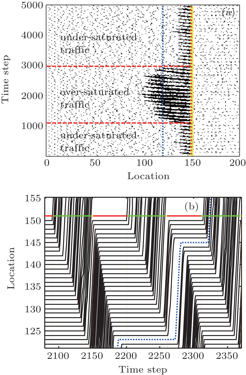
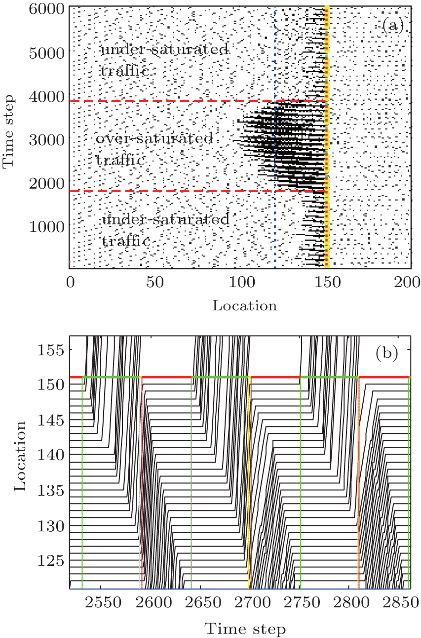
1) Time-delayed traffic breakdown Figure 2 presents the typical spatiotemporal pattern of traffic flow obtained from two independent runs with the slow-to-start behavior and the inch-forward behavior activated by setting p_gm = 0.1, p_max = 0.6, p_ym = 0, p_ys = 0, p_rm1 = 0, p_rm0 = 0.01, and p_rs = 0, respectively. The slow-down behavior is inactivated by allowing the velocity increment to vary in the range − b_max ≤ δ _k ≤ a_max. The traffic flow is initially under-saturated, but it transits into the over-saturated traffic after the breakdown at approximately 1541^th step (15^th cycle) in Fig. 2(a) and 3631^th step (33^th cycle) in Fig. 2(b), respectively. By performing a number of independent runs, it can be found that the transition to the over-saturated traffic occurs after a random delay. This spontaneous traffic breakdown has been recently documented in Refs. [12], [17]– [20].

Fig. 2.

	Figure Option ViewDownloadNew Window
	Fig. 2. The spatiotemporal pattern of traffic flow obtained from two independent runs. The effective section is bounded by the effective point and the traffic light whose locations are denoted by the two vertical lines from left to right. (a) One realization, (b) another realization.

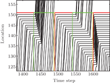
In order to see the movement change before and after the breakdown in a microscopic way, the trajectories corresponding to the traffic shown in Fig. 2(a) are plotted for the two cycles just before and after the breakdown and shown in Fig. 3. Before the traffic breakdown, the queue formed at the signal can be fully dissolved during the green phase and each vehicle closely follows its predecessor after the onset of the green signal, resulting in rapid queue dissolution. However, in the next green phase, the delayed start can be observed for a number of vehicles in the queue. This delayed start increases the stopped time and decreases the number of vehicles passing the traffic light accordingly. As the probability p_gs is linearly proportional to the stopped time, the increase of the stopped time will result in an increase of p_gs which is primarily responsible for the slow-start. In such way, the queue accumulatively extends step by step.

Fig. 3.

	Figure Option ViewDownloadNew Window
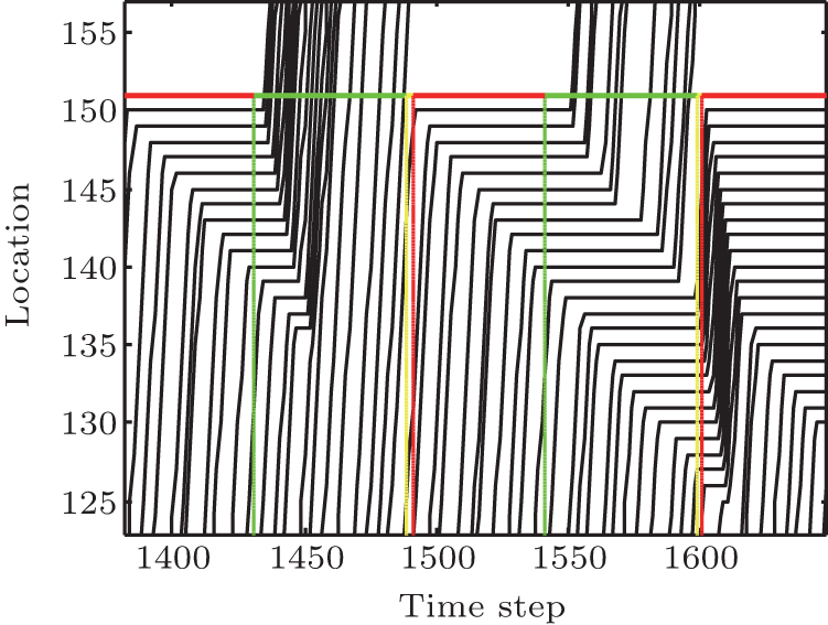	Fig. 3. Trajectories for the two cycles where the traffic transits from under-saturated state into over-saturated state. The upper horizontal line denotes the location of the traffic light.

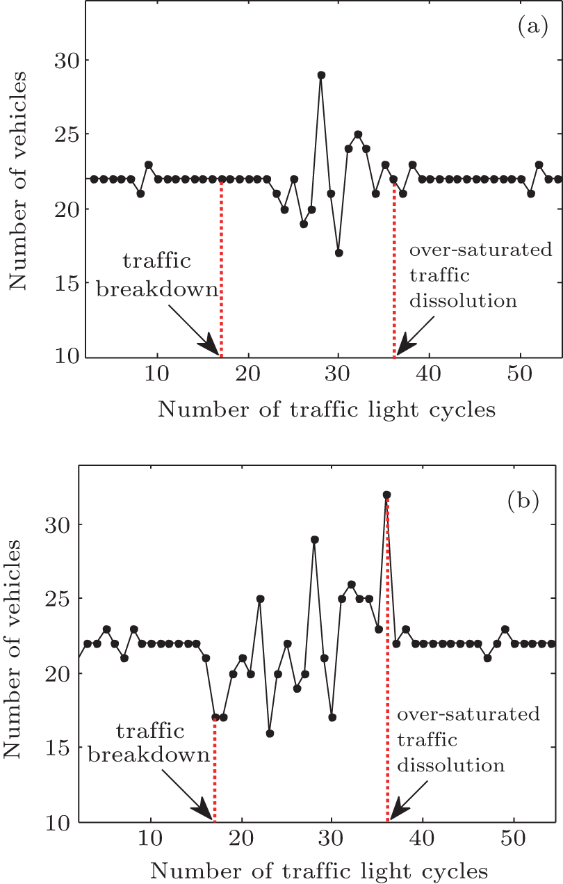
To further investigate the spontaneous breakdown, three parameters (i.e., number of vehicles, velocity, and time headway) for the traffic shown in Fig. 2(a) have been collected by using two virtual detectors located at the effective point and the traffic light, and the results averaged for each cycle are presented in Figs. 4– 6.

Fig. 4.

	Figure Option ViewDownloadNew Window
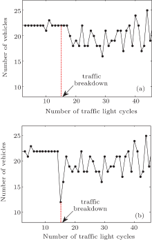
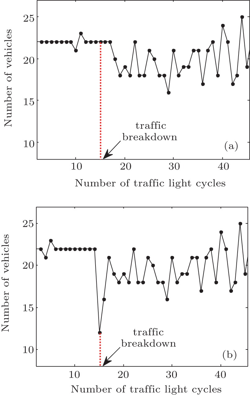	Fig. 4. Number of vehicles crossing the effective point (a) and the traffic light (b) in each traffic light cycle, corresponding to Fig. 2(a).

Fig. 5.

	Figure Option ViewDownloadNew Window
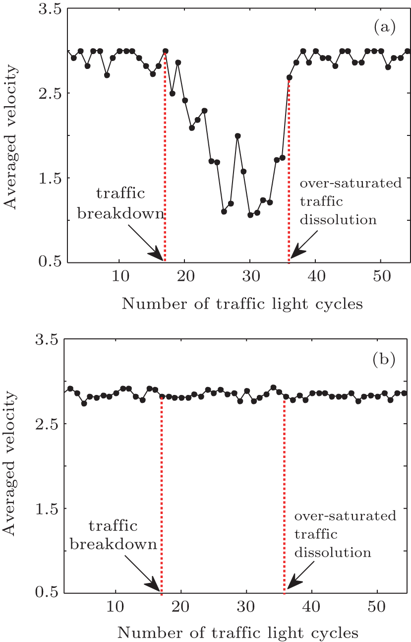
	Fig. 5. Averaged velocity of the vehicles crossing the effective point (a) and the traffic light (b) in each traffic light cycle, corresponding to Fig. 2(a).

Fig. 6.

	Figure Option ViewDownloadNew Window
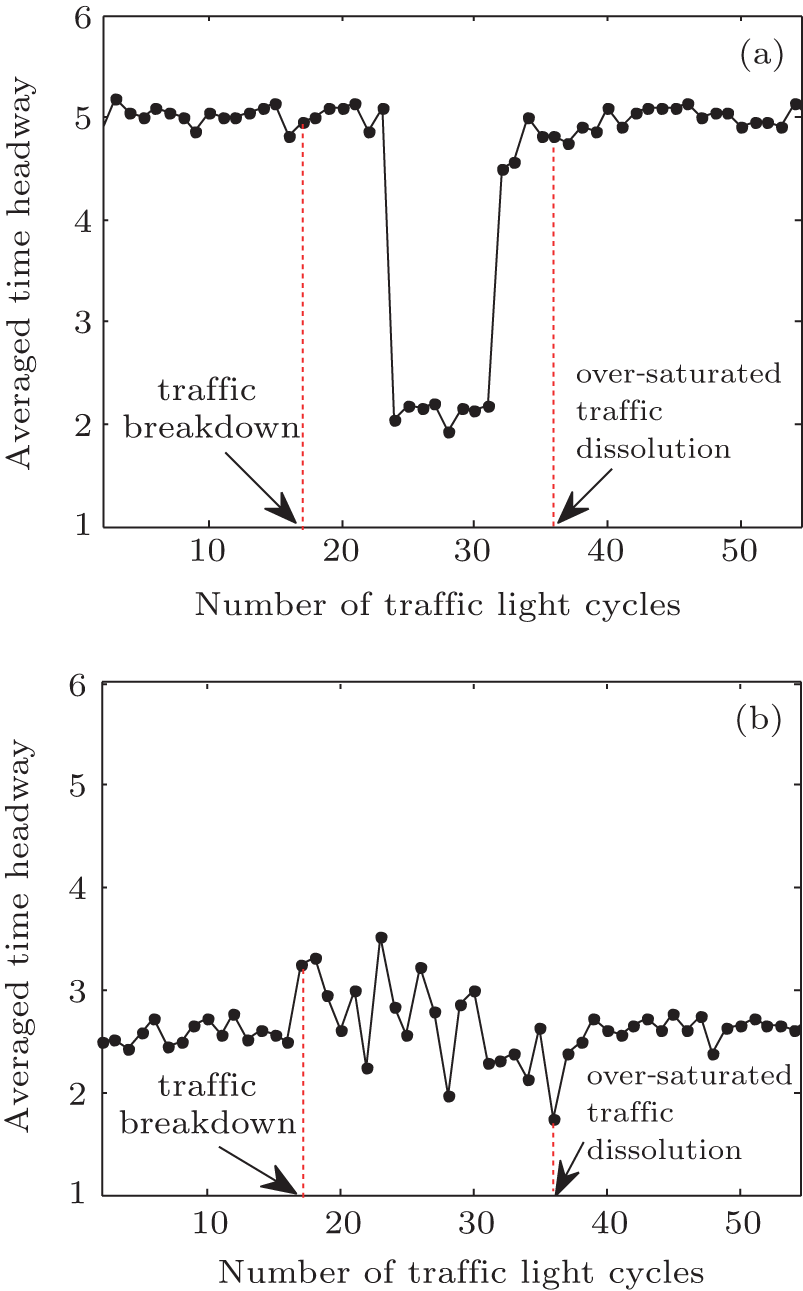
	Fig. 6. Averaged time headway of the vehicles crossing the effective point (a) and the traffic light (b) in each traffic light cycle, corresponding to Fig. 2(a).

A small variation on the number of vehicles crossing the effective point can be observed from Fig. 4(a) for the period before breakdown; the averaged number is approximately 22 (equivalent to 720 vehicles/h). On the contrary, the fluctuation becomes strong after the traffic transits to be over-saturated. Although the results shown in Figs. 4(a) and 4(b) have a similar pattern and the fluctuations are in the same order before and after the breakdown, there is a difference that a drop in the number of vehicles can be observed at the traffic breakdown cycle in Fig. 4(b) but the drop is delayed for a couple of cycles in Fig. 4(a). The drop in the number of vehicles passing the traffic light is largely resulted from the delayed start as evidenced by the averaged time headway presented in Fig. 6(b). The influence of the changes in the number of vehicles passing the traffic light will propagate upstream and therefore the number of vehicles passing the effective point will be affected with a time delay.

Figure 5(a) shows the averaged velocities when the vehicles crossing the effective point. In the under-saturated traffic, the velocities averaged for each cycle is either maximum or near-maximum and the velocity variation is small. However, in the over-saturated traffic, the velocity decreases to almost 2 cell/step on average and the fluctuation becomes strong. On the other hand, the result in Fig. 5(b) implies that the breakdown has little influence on the averaged velocity of the vehicles crossing the traffic light and the fluctuation throughout the test period is smaller than that in Fig. 5(a). The small variation on the velocity indicates the outflow rate from the queue formed before the light turns to be green is constant and independent to whether the queue can be fully discharged during green time.

The time headway has been measured and averaged only for the vehicles that passed the effective point or the traffic light in each cycle. In other words, if a vehicle cannot cross the effective point or the traffic light during the current cycle, the time headway will not be included. In Fig. 6(a), before the breakdown, the averaged time headway is around 5 cells (25 m), approximately equivalent to the inflow rate of 0.2 vehicles/step. A sharp drop of the time headway can be observed after the breakdown for three cycles. The averaged time headway in the over-saturated traffic is around 2 cells (10 m). However, the situation is different when the vehicles are crossing the traffic light. At the breakdown cycle, the averaged time headway is increased sharply, implying there is a considerable time loss due to the slow start. Consequently, the time loss causes a delay in the process of queue dissolution and some vehicles have to wait in front of the traffic light for another cycle (see Fig. 3). After the traffic breakdown, the fluctuation gradually becomes strong.

From Fig. 2(a), it can be seen that the upstream of the queue extends quickly into section A after the traffic breakdown. When the vehicle previously stopped in front of the effective point accelerates and crosses the effective point, the velocity, shown in Fig. 6(a), is generally small as it cannot accelerate to the maximum value within one time step. The vehicle stopped on section A will immediately accelerate with high probability (due to P_n = 0.1) as long as its front cell becomes free. This results in a small gap (headway is around 2 cells in Fig. 6(a)) between two successive vehicles.

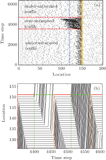
To verify the influence of the slow-to-start behavior on the traffic breakdown, this behavior was initially activated but inactivated by setting p_gs = p_gm after the traffic breakdown. However, during the test period, the inch-forward behavior is always on but the slow-down behavior off. Figure 7(a) shows the transition from the initial under-saturated state into the over-saturated state when the slow-to-start behavior is incorporated in the model, but the transition is reversed when the behavior is off. The trajectories shown in Fig. 7(b) correspond to the traffic flow in Fig. 7(a) for the period when the slow-to-start behavior is switched off at the 4511^th step. It is apparent that after the slow-to-start behavior is off the start delay is eliminated, resulting in a closely following pattern when the vehicles pass the traffic light.

Fig. 7.

	Figure Option ViewDownloadNew Window
	Fig. 7. The spatiotemporal pattern of traffic flow (a) and the trajectories for the two cycles just before and after the slow-to-start behavior is inactivated (b).

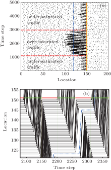
In addition, we have examined the influence of the inch-forward behavior on the traffic breakdown in the same way. The inch-forward behavior is isolated from the slow-to-start behavior by changing the inch-forward behavior (i.e., p_rs is changed from 0 to 0.8) but fixing the other during the test period. The traffic shown in Fig. 8(a) is initially under-saturated but changed to be over-saturated after the traffic breakdown. Then, p_rs is changed from 0 to 0.8 at the 2201^th step and the queue begins to dissolve gradually. The trajectory marked as the dotted line in Fig. 8(b) indicates that, after p_rs is changed from 0 to 0.8, the vehicle originally stopped at the 123^th cell is still motionless even though there is a big gap to the preceding vehicle during the red phase. After a while, the vehicle starts to move toward the traffic light and stops in front of the queue. This movement can reduce the queuing time for the vehicle and consequently the probability for the slow start. Then, the decrease of the slow start phenomenon can help the queue dissolution.

Fig. 8.

	Figure Option ViewDownloadNew Window
	Fig. 8. The spatiotemporal pattern of traffic flow (a) and the trajectories for the two cycles just before and after prs is changed from 0 to 0.8 (b).

2) Dissolution of over-saturated traffic If the slow-down behavior is incorporated into the model, we have found that the traffic transits from over-saturation into under-saturation, promoting the queue dissolution. Figure 9(a) shows the traffic obtained when the slow-down behavior was activated by setting p_rm0 = 0.01 and p_rm1 = 1, after the over-saturated traffic lasted for eight cycles. Before activating the slow-down behavior, the traffic breakdown occurs at approximately the 1761^th step (17^th cycle), which was realized using the same setting as that in the last subsection with the slow-down behavior inactivated. Figure 9(b) shows the trajectories for the three cycles when the slow-down behavior was activated at the 2641^th step (the 25^th cycle). By a close observation on the movements for each red phase, it can be found that the velocity is relatively lower after the slow-down behavior was switched on. The low velocity prolongs the moving time and thus shortens the queueing time. As a result, the probability for the slow-to-start behavior is also reduced, as the probability is linearly dependent on the stopped time. In such a way, the queue can be gradually dissolved with the assistance of the slow-down behavior.

Fig. 9.

	Figure Option ViewDownloadNew Window
	Fig. 9. The spatiotemporal pattern of traffic flow (a) and the trajectories for the three cycles when the slow-down behavior is activated at the 2641th cycle (b).

Figure 10 shows the number of vehicles passing the effective point and the traffic light in each cycle. The result shown in Fig. 10(a) indicates the number of vehicles driving through the effective points is around 22 on average and the variation is relatively small, in under-saturated traffic. After the traffic breakdown for six cycles, the number begins to fluctuate strongly, with the maximum of 29 and the minimum of 17.

Fig. 10.

	Figure Option ViewDownloadNew Window
	Fig. 10. Number of vehicles crossing the effective point (a) and the traffic light (b) in each traffic light cycle, corresponding to Fig. 9.

Figure 10(b) shows the number of the vehicles crossing the traffic light is relatively constant and 22 on average in under-saturated traffic. However, the number drops to 17 when the traffic breakdown occurs at the 17^th cycle and the number reaches to the maximum when the traffic transits from the over-saturation to the under-saturation. The reason for the delayed fluctuation after the breakdown in Fig. 10(a) is that it takes some time to propagate the influence of the breakdown from the traffic light to the effective point.

The velocities averaged for each cycle, when the vehicles crossing the effective point and the traffic light, are shown in Fig. 11. While figure 11(a) shows a down concave curve in general, the result in Fig. 11(b) fluctuates slightly. As shown in Fig. 11(a), the driving velocity is near to the maximum in under-saturated traffic, indicating a free flow around the effective point. The minimum value in over-saturated traffic is close to a 1 cell/step. The result in Fig. 11(b) indicates the vehicles passed the traffic light at high velocity and the fluctuation is weak through the test period.

The averaged time headway shown in Fig. 12(a) is approximately 5 cells for under-saturated traffic. After traffic breakdown for six cycles, the time headway goes down firstly, then varies slightly, and finally bounces up before the traffic transits into under-saturated traffic. On the contrast, there is no apparent pattern in the result shown in Fig. 12(b), even though the fluctuation is generally stronger in the over-saturated traffic than that in the under-saturated traffics.

Fig. 11.

	Figure Option ViewDownloadNew Window
	Fig. 11. Averaged velocity of vehicles crossing the effective point (a) and the traffic light (b) in each traffic light cycle, corresponding to Fig. 9.

Fig. 12.

	Figure Option ViewDownloadNew Window
	Fig. 12. Averaged time headway of vehicles crossing the effective point (a) and the traffic light (b) in each traffic light cycle, corresponding to Fig. 9.

The drop in the number after the breakdown shown in Fig. 10(b) can be explained by the slow-to-start effect as stated in the previous subsection. After activating the slow-down behavior, the vehicles will reduce their velocities during the red phases, even if it is not necessary to decelerate to avoid traffic violation and collision. With the slow-down behavior, the vehicles will take a longer time to reach the queue end, resulting in a reduced queuing time. As a result, the probability for the slow start will be reduced accordingly. As shown in Fig. 12(b), the small time headways around the transition from over-saturation to under-saturation indirectly show some evidence for the reduced slow start effect. This means that the queuing vehicles will start their movements with less delay and the number of vehicles passing the traffic light will be increased. Consequently, the slow-down behavior alleviates the tendency of the queue growing. The growing rate of the queue is effectively suppressed but the discharging rate is not altered, resulting in the queue shrinking step by step. This may account for why the slow-down behavior can help dissolve the over-saturated traffic.

To evaluate the influence of different behaviors on traffic breakdown, we have performed a number of simulations by varying the probabilities. Figures 13(a) and 13(b) present the percentage and the averaged cycle at which the traffic broke down within 30 cycles and each has been averaged over 300 independent runs.

Fig. 13.

	Figure Option ViewDownloadNew Window
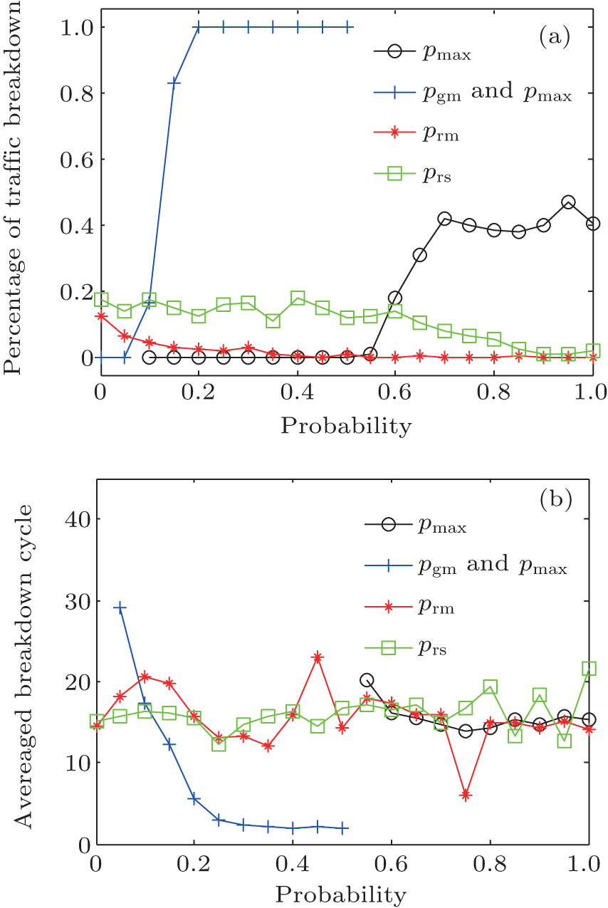	Fig. 13. Percentage of traffic breakdown (a) and the averaged breakdown cycle (b) for different probabilities.

When examining the slow-to-start behavior, p_max has been firstly varied from 0.1 to 1 with an interval of 0.05, but p_gm fixed to be 0.1. Note that p_max should be larger in order to activate the slow-to-start behavior according to R3 for the vehicles on the effective section. By observing the percentage of traffic breakdown and the averaged breakdown cycle, it is clear that traffic breakdown never occurs during the test period when p_max is less than 0.55. When p_max increases from 0.55 to 0.7, the percentage increases gradually but the breakdown cycle decreases. When p_max is greater than 0.7, the percentage and breakdown cycle fluctuate slightly. Secondly, p_gm and p_max have been varied synchronously, so that the difference between them is always 0.5. In this way, the number of vehicles that manifest the slow-to-start behavior is mainly affected by the probability, p_gm. Note that p_gm is bounded at 0.5 when it increases from 0, as p_max reaches to 1 at that time. The result shown with the marker ‘ + ’ in Fig. 13(a) indicates that the percentage of traffic breakdown is an increasing function of p_gm. However, the breakdown cycle decreases to 2 when p_gm is larger than 0.35. In short, the slow-to-start behavior potentially promotes traffic breakdown.

Next, p_rm1 has been varied but p_rm0 fixed to 0.01 in order to generate the slow-down behavior with a different degree. The line with the marker ^{‘ * ’} in Fig. 13(a) shows a decreasing tendency in the percentage of the traffic breakdown as p_rm1 increases, indicating the probability of traffic breakdown can be reduced if the slow-down behavior is constantly reinforced. The result shown in Fig. 13(b) indicates that the traffic breakdown cycle is not significantly affected by p_rm1.

The final examination has been made by varying p_rs so as to realize the inch-forward behavior with a different degree. The result shown in Fig. 13(a) with the marker ‘ ☐ ’ indicates a general flat pattern when p_rs is less than 0.4 and a slow-decreasing pattern when p_rs is greater than 0.4. On the other hand, there is no apparent pattern for the breakdown cycle when p_rs increases. Note that the larger p_rs is, the more inactive is the inch-forward behavior. The result implies that traffic breakdown is likely to be affected negatively by the inch-forward behavior, even though the influence is not significant.