Hybrid natural element method for large deformation elastoplasticity problems<xref ref-type="fn" rid="cpb142378fn1">*</xref>

Cite this Article

Ma Yong-Qi, Zhou Yan-Kai. Hybrid natural element method for large deformation elastoplasticity problems* . Chinese Physics B, 2015, 24(3): 030204 Copy to clipboard

Permissions

Hybrid natural element method for large deformation elastoplasticity problems*

Ma Yong-Qi^a),^b)†, Zhou Yan-Kai^a)

a)Shanghai Institute of Applied Mathematics and Mechanics, Shanghai University, Shanghai 200072, China

b)Department of Mechanics, Shanghai University, Shanghai 200444, China

^†Corresponding author. E-mail: mayq@staff.shu.edu.cn

^*Project supported by the Natural Science Foundation of Shanghai, China (Grant No. 13ZR1415900).

Abstract

We present the hybrid natural element method (HNEM) for two-dimensional elastoplastic large deformation problems. Sibson interpolation is adopted to construct the shape functions of nodal incremental displacements and incremental stresses. The incremental form of Hellinger–Reissner variational principle for elastoplastic large deformation problems is deduced to obtain the equation system. The total Lagrangian formulation is used to describe the discrete equation system. Compared with the natural element method (NEM), the HNEM has higher computational precision and efficiency in solving elastoplastic large deformation problems. Some numerical examples are selected to demonstrate the advantage of the HNEM for large deformation elastoplasticity problems.

Keyword: 02.60.Cb; 02.60.Lj; 46.15.–x; hybrid natural element method; large deformation elastoplasticity; Hellinger–Reissner variational principle; meshless method

Show Figures

1. Introduction

In solving the large deformation problems, the finite element method (FEM) may encounter difficulties when adaptive meshing or rezoning techniques may be helpful, but they are not widely used because of their complexity and imperfections. On the contrary, the meshless method is a numerical method based on nodes, which does not need to generate mesh, so adaptive meshing or rezoning techniques are not used in the meshless method.^[1] Therefore, the meshless method has some advantages in handling large deformation problems.

Many meshless methods have been developed, such as the element-free Galerkin method, ^{[2– 4]} improved element-free Galerkin method, ^{[5– 8]} complex variable meshless method, ^{[9– 11]} complex variable element-free Galerkin method, ^{[12– 16]} interpolating element-free Galerkin method, ^{[17, 18]} radial basis function method, ^[19] finite point method, ^{[20, 21]} meshless local Petrov– Galerkin method, ^[22] reproducing kernel particle method, ^{[23– 27]} meshless manifold method, ^{[28, 29]} boundary element-free method, ^{[30– 38]} and the improved boundary element-free method.^{[39– 42]}

Braun and Sambridge presented another meshless method, namely, the natural element method.^[43] Many researchers applied the NEM to solve mechanical problems. Sukumar et al.^[44] used the NEM to analyze two-dimensional small displacement elastostatics. Bueche et al.^[45] investigated the performance of NEM in two-dimensional linear elastodynamics. Cueto et al.^[46] employed the NEM for two-dimensional and three-dimensional piece-wise homogeneous domains. Martí nez et al.^[47] simulated flows involving short fiber suspensions with the NEM. Calvo et al.^[48] solved large strain hyperelastic problems using the NEM. Daneshmand and Niroomandi discussed the vibration modes of fluid-structure systems with the NEM.^[49] Daneshmand et al.^[50] calculated two-dimensional flow under sluice gates using the NEM. Shahrokhabadi et al.^[51] developed the NEM to solve seepage problems. Cho et al.^[52] established the NEM of Reissner– Mindlin plate for a locking-free numerical analysis of plate-like thin elastic structures. Different from the NEM, the HNEM adopts displacement approximation and stresses approximation respectively to obtain the discrete equation system with the Hellinger– Reissner variational principle. The HNEM has been used to solve the elasticity problems and elastoplastic problems.^{[53, 54]}

Various meshless methods have been developed for large deformation analysis of non-linear materials and structures. Chen et al.^[55] analyzed non-linear elastic and inelastic structures based on reproducing kernel particle methods. Li et al.^[56] studied mesh-free simulations of shear banding in large deformation. Ren et al.^[57] modelled the superelastic behaviour of shape memory alloys using the element-free Galerkin method. Liew et al.^[58] analyzed the pseudoelastic behavior of an SMA beam by the element-free Galerkin method. Liew et al.^[59] developed an FSDT and a meshfree method for corrugated plates. Naffa and Al-Gahtani discussed the radial basis function method for large deflection of thin plates.^[60] Rossi and Alves investigated a modified element-free Galerkin method and applied it to large deformation processes.^[61] Zhao and Liew applied the element-free kp-Ritz method to functionally graded plates.^[62] Doweidar et al.^[63] adopted the implicit and explicit natural element methods to analyze large strains of soft biological tissues. Li et al.^{[64– 66]} proposed complex variable element-free Galerkin methods for large deformation problems. Peng et al.^[67] used the FSDT and the moving least-squares approximation to analyze ribbed rectangular plates.

Based on the Sibson interpolation, the HNEM for two-dimensional elastoplastic large deformation problems is discussed in this paper. The incremental formulation of the Hellinger– Reissner variational principle is deduced to obtain the incremental equation system. The total Lagrangian formulation is used to describe this equation system. The Mises yield criterion is adopted as yield condition and the linear hardening elastoplastic model is used as the flow rule. The corresponding formulae are solved by the Newton– Raphson iteration method with displacement convergence criterion. Some numerical examples of large deformation elastoplasticity problems are computed by the HNEM.

2. Basic equations of large deformation elastoplasticity problems

2.1. Incremental formulation of Hellinger– Reissner variational principle for large deformation elastoplasticity problems

We adopt the total Lagrangian formulation to describe the large deformation problems, i.e., the original configuration is used as reference configuration. For a question domain ⁰Ω , suppose that displacement , strain , and stress at time t have been obtained, and body force on ⁰Ω , boundary force on , and boundary displacement on at time t + Δ t are given. Then displacement , strain , and stress at time t + Δ t can be obtained after incremental displacement ₀u_i, incremental strain ₀ε _ij, and incremental stress ₀σ _ij are computed from t to t + Δ t.

The incremental formulation of the Hellinger– Reissner variational principle can be expressed as^[68]

where B is the incremental surplus energy density function

with ₀C_ijkl being the relationship between stress increment ₀σ _ij and strain increment ₀ε _ij,

It must be pointed out that the linear relationship supposed here is true only for an infinitesimal increment.

The decomposition of incremental strain ₀ε _ij can be written as

where ₀e_ij and ₀η _ij are the linear and quadratic terms of the incremental strain ₀ε _ij, respectively. Namely,

where

Then equation (1) can be rewritten as

For further linearization, ₀σ _ij0η _ij in the third integral term in Eq. (9) needs to be omitted. Suppose the displacement boundary condition was satisfied, then equation (9) can be rewritten as

Thus, the incremental formulation of the Hellinger– Reissner variational principle to deduce the HNME for large deformation elastoplasticity problems is found.

2.2. Two-dimensional elastoplastic constitution relationship

For an isotropic hardening material, the incremental form of the stress– strain relation in plane problems can be expressed as

We adopt the Mises yield criterion to judge whether an arbitrary point of the material is in the plastic state. When equivalent stress σ _l of a point is greater than yield stress σ _s of the material, then this point is in plastic state; otherwise it is in elastic state. The equivalent stress σ _l of an arbitrary point can be written as

If the point is in elastic state, ₀C^e of this point is

where

When the point is in the plastic state, for plane stress problems, ₀C^ep of this point is

and for plane strain problems, ₀C^ep of this point is

where E is Young’ s modulus, ν is Poisson’ s ratio, and H′ is the plastic modulus for material hardening, and

E′ is known as the tangent modulus. S₁₁ and S₂₂ are the deviatoric stresses, and

In Eqs. (16) and (17),

3. The HNEM for elastoplastic large deformation problems

3.1. Sibson interpolation

The Sibson interpolation is based on the well-known Voronoi diagram and Delaunay tessellation. Suppose a set of scattered nodes N = {N₁, N₂, … , N_m} in R², the nodal coordinates are x_i (i = 1, 2, … , m). The Voronoi diagram T(N) of the set N is a subdivision of the domain into Voronoi cells T(N_i), and the Voronoi cell T(N_i) is defined as

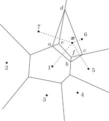
where d(x_i, x_j) is the distance between x_i and x_j. The Delaunay triangulation is the dual of the Voronoi diagram, which is constructed by connecting the nodes whose Voronoi cells have common boundaries. The circumcircles of Delaunay triangles, known as natural neighbour circumcircles, can be used to find the natural neighbour nodes of x. In other words, if x lies within the natural neighbour circumcircle of triangle DT(N_i, N_j, N_k), then N_i, N_j, and N_k are the natural neighbour nodes of x. The Voronoi diagram, the Delaunay triangulation, and natural neighbour circumcircles of a set N are shown in Fig. 1, in which we can find that nodes 1, 5, 6, 7 are the natural neighbor nodes of x.

	Figure Option View Download New Window
	Fig. 1. Voronoi diagram T(N), Delaunay triangulation DT(N), and natural neighbour circumcircles.

The Sibson interpolation shape function of x with respect to a natural neighbour x_i is defined as

where n is the number of natural neighbours of x, A_i (x) is the area of overlap of Voronoi cell T(x_i) and Voronoi cell T(x), and A(x)is the area of Voronoi cell T(x ).

Referring to Fig. 2, the Sibson interpolation shape function ϕ ₅ (x) is

	Figure Option View Download New Window
	Fig. 2. Voronoi cell T(x).

The derivatives of the shape functions can be obtained by differentiating Eq. (27)

The displacement approximations u^h(x) of point x can be expressed as

where u_i is the displacement vector of node i.

According to definition of the shape function (27), the following remarkable properties is self-evident:

Equation (33) shows that the shape functions possess the Kronecker delta function property, therefore the essential boundary conditions can be implemented directly as in the FEM. Equations (34) and (35) define a partition of unity and linear completeness, which imply that the shape functions can reproduce the rigid body displacement and the constant strain.

3.2. The HNEM for two-dimensional elastoplastic large deformation problems

Suppose there are n nodes in the two-dimensional solution domain ⁰Ω , from Sibson interpolation approximations (Eq. (31)), the incremental displacement vector ₀u(x) and the incremental stress vector ₀σ (x) from t to t + Δ t at any point x in the domain ⁰Ω can be written as

where ₀Φ (x) and ₀P(x) are the matrix form of shape functions

and ϕ _i is the shape function of x with respect to node x_i, which can be constructed by Eq. (27), ₀q and ₀β are the nodal incremental displacement vector and the nodal incremental stress vector, respectively,

The matrix form of Eq. (4) in the two-dimensional problems is

where

Thus, equation (10) can be expressed as

where ₀C can be obtained by Eqs. (13), (16), and (17).

Substitute Eqs. (36) and (37) into Eq. (51), we can obtain

Based on stationary value condition of multi-variation variation principle, i.e.,

and we can obtain

Substituting Eq. (54) into Eq. (52), we obtain

According to the stationary condition of variation principle, i.e.,

the following equations can be obtained:

where

The above is the HNEM for two-dimensional elastoplastic large deformation problems. The Newton– Raphson method can be adopted to solve Eq. (57).

4. Numerical examples

In this section, several examples are presented to illustrate the applicability of the HNEM for two-dimensional elastoplastic large deformation problems. The results of these examples are obtained by using the HNEM, NEM, and Abaqus. Delaunay triangles are used as integration cells, gauss integration is adopted as integration scheme, and three Gauss points are used in each integration cell. The loads in these examples do not vary with the configuration of the object.

4.1. Cantilever beam with a concentrated force

Consider a cantilever beam subjected to a concentrated force, the left side is clamped, as shown in Fig. 3. The concentrated force is p = 10 N, length of the beam is L = 10 m, height is H = 1 m, and the unit thickness of the beam is considered. Elasticity modulus and Poisson’ s ratio are E = 1.2× 10⁴ Pa and ν = 0.2, respectively. The yield stress is σ _s = 480 Pa and E′ = 0.2E. Regardless of the gravity, the beam can be discussed as a plane stress problem.

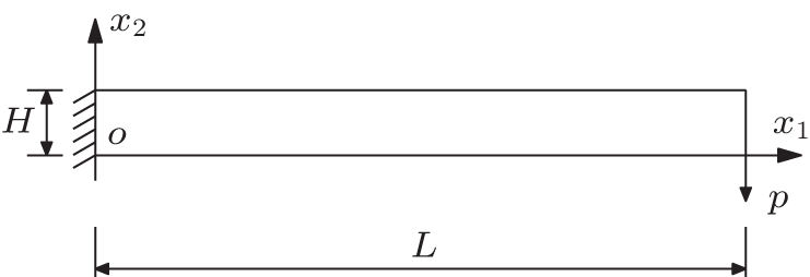	Figure Option View Download New Window
	Fig. 3. Cantilever beam with a concentrated force.

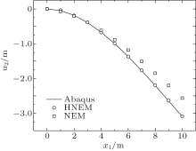
As shown in Fig. 4, 55 nodes and 80 Delaunay triangles are distributed on the cantilever beam. One hundred steps are adopted to apply the load. The nodal vertical displacements, at the axis of the cantilever beam, are shown in Figs. 5 and 6. Under the same nodal layout, the results from the HNEM agree better with those from the Abaqus than the ones from the NEM, as shown in Fig. 5. Under a similar numerical precision, the CPU time used in the HNEM is less than that in the NEM, as shown in Fig. 6.

	Figure Option View Download New Window
	Fig. 4. Nodal distribution and Delaunay triangles of the cantilever beam.

	Figure Option View Download New Window
	Fig. 5. Vertical displacements of the nodes at the axis of the cantilever beam.

	Figure Option View Download New Window
	Fig. 6. Vertical displacements of the nodes at the axis of the cantilever beam and the comparison of the CPU time between the HNEM and the NEM.

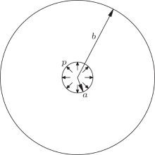
4.2. Cylinder under a distributed inner pressure

A thick walled cylinder under a distributed inner pressure is considered, as shown in Fig. 7. The inner pressure is p = 1000 Pa, and the radiuses are a = 1 m and b = 5 m. The elasticity modulus and Poisson ratio are E = 1.0 × 10⁵ Pa and ν = 0.25, respectively. The yield stress is σ _s = 150 P, and E′ = 0.2E. The cylinder can be discussed as a plane strain problem without considering the body force.

	Figure Option View Download New Window
	Fig. 7. Cylinder under a distributed inner pressure.

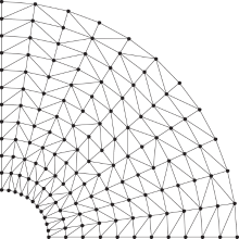
Consider the symmetry of the cylinder, only a quarter of the cylinder needs to be calculated, as shown in Fig. 8. Figure 9 shows 144 nodes with corresponding Delaunay triangles used for solution. The number of the whole load steps is set as 100. The nodal horizontal displacements at x₂ = 0 obtained using the HNEM and NEM are shown in Fig. 10. It can be seen that, under the condition of the same nodal layout, the results attained by the HNEM are closer to that using Abaqus than ones using the NEM.

	Figure Option View Download New Window
	Fig. 8. A quarter of the cylinder with boundary conditions.

	Figure Option View Download New Window
	Fig. 9. Nodal distribution and Delaunay triangles of a quarter of the cylinder.

	Figure Option View Download New Window
	Fig. 10. Horizontal displacements of nodes at x₂ = 0 of the cylinder.

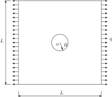
4.3. Square plate with a central hole subjected to an axial uniform tension

A square plate with a central hole subjected to an axial uniform tension is shown in Fig. 11. The axial uniform tension is q = 1000 N/m, the length is L = 10 m, and the radius of the hole is R = 1 m. The elasticity modulus and Poisson ratio are E = 1.0 × 10⁵ Pa and ν = 0.25, respectively. The yield stress is σ _s = 400 Pa and E′ = 0.2E. The unit thickness of the plate is considered. Regardless of the body force, the plate can be calculated as a plane stress problem.

	Figure Option View Download New Window
	Fig. 11. A square plate with a central hole subjected to an axial uniform tension.

As shown in Fig. 12, only a quarter of the square plate needs to be considered. 99 nodes and the corresponding Delaunay triangles are distributed on a quarter of the square plate, as shown in Fig. 13. 200 steps are adopted to apply the load. With the same nodal distribution, the nodal horizontal displacements of the plate at x₂ = 5 m obtained from the HNEM and the NEM are shown in Fig. 14. It can be observed that the results from the HNEM are in better agreement with the ones from the Abaqus than those from the NEM.

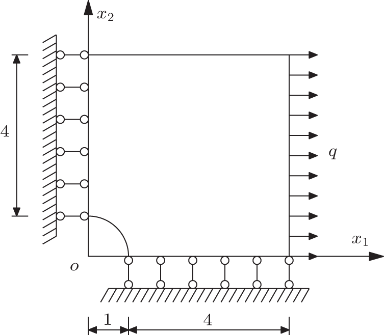	Figure Option View Download New Window
	Fig. 12. A quarter of the square plate with boundary conditions.

	Figure Option View Download New Window
	Fig. 13. Nodal distribution and Delaunay triangles of a quarter of the square plate.

	Figure Option View Download New Window
	Fig. 14. Nodal horizontal displacements of the plate at x₂ = 5m.

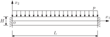
4.4. Clamped beam under a distributed load

The final example is a beam, which is fixed at both ends and subjected to a distributed load, as shown in Fig. 15. The length of the beam is L = 10 m, height is H = 1 m, and the unit thickness of the beam is considered. The distributed load is p = 50 N/m. The elasticity modulus is E = 1.2 × 10⁴ Pa, Poisson’ s ratio is ν = 0.2, the yield stress is σ _s = 480 Pa, and E′ = 0.2E. The beam can be discussed as a plane stress problem without considering the gravity.

	Figure Option View Download New Window
	Fig. 15. Clamped beam under a distributed load.

We adopt 55 nodes and 80 Delaunay triangles for this example, as shown in Fig. 16. The number of load steps is 100. The vertical displacements of nodes at the axis of the beam obtained by the HNEM and NEM are shown in Figs. 17 and 18. From Fig. 17, we can see that, under the same nodal distribution, the results obtained by using the HNEM agree better with the ones using the Abaqus than the ones using the NEM. It can be observed from Fig. 18 that the CPU time spent in the HNEM is less than that in the NEM under a similar numerical precision. This demonstrates that the HNEM has a higher computational efficiency than the NEM.

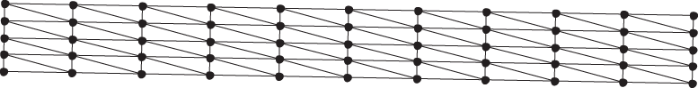	Figure Option View Download New Window
	Fig. 16. Nodal distribution and Delaunay triangles of the clamped beam.

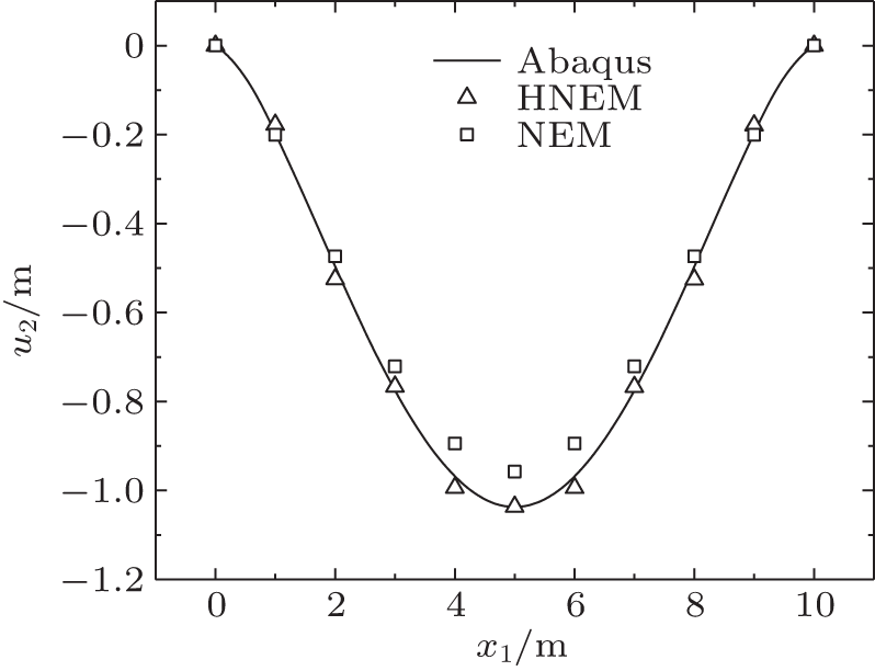	Figure Option View Download New Window
	Fig. 17. Vertical displacements of the nodes at the axis of the clamped beam.

	Figure Option View Download New Window
	Fig. 18. Vertical displacements of the nodes at the axis of the clamped beam and the comparison of the CPU time between the HNEM and the NEM.

5. Conclusions

The HNEM for analyzing large deformation elastoplasticity problems is discussed in this paper. The Sibson interpolation shape functions are chosen as the trial and test functions of nodal incremental displacements and incremental stresses. The incremental formulation of Hellinger– Reissner variational principle suitable for elastoplastic large deformation problems is deduced to obtain the incremental discrete equations, and these equations are solved by the Newton– Raphson iteration method. Some numerical examples of large deformation elastoplasticity problems show that the results of the HNEM have higher computational precision and efficiency than the ones of the NEM.

Reference

View Option

1	Onishi Y and Amaya K 2012 Int. J. Numer. Meth. Eng. 92 36 DOI:10.1002/nme.v92.1 [Cited within:1] [JCR: 2.056]
2	Belytschko T, Lu Y Y and Gu L 1994 Int. J. Numer. Meth. Eng. 37 229 DOI:10.1002/(ISSN)1097-0207 [Cited within:1] [JCR: 2.056]
3	Wang J F, Sun F X and Cheng R J 2010 Chin. Phys. B 19 060201 DOI:10.1088/1674-1056/19/6/060201 [Cited within:1] [JCR: 1.148] [CJCR: 1.2429]
4	Cheng R J and Cheng Y M 2011 Chin. Phys. B 20 070206 DOI:10.1088/1674-1056/20/7/070206 [Cited within:1] [JCR: 1.148] [CJCR: 1.2429]
5	Zhang Z, Liew K M and Cheng Y 2008 Engin. Anal. Bound. Elem. 32 100 DOI:10.1016/j.enganabound.2007.06.006 [Cited within:1] [JCR: 1.596]
6	Zhang Z, Liew K M, Cheng Y and Lee Y Y 2008 Engin. Anal. Bound. Elem. 32 241 DOI:10.1016/j.enganabound.2007.08.012 [Cited within:1] [JCR: 1.596]
7	Zhang Z, Hao S Y, Liew K M and Cheng Y M 2013 Engin. Anal. Bound. Elem. 37 1576 DOI:10.1016/j.enganabound.2013.08.017 [Cited within:1] [JCR: 1.596]
8	Zhang Z, Wang J, Cheng Y and Liew K M 2013 Sci. China-Phys. Mech. Astron. 56 1568 DOI:10.1007/s11433-013-5135-0 [Cited within:1]
9	Cheng Y M and Li J H 2005 Acta Phys. Sin. 54 4463(in Chinese) http://118.145.16.217/magsci/article/article?id=17384908 [Cited within:1] [JCR: 1.016] [CJCR: 1.691]
10	Wang J F and Cheng Y M 2012 Chin. Phys. B 21 120206 DOI:10.1088/1674-1056/21/12/120206 [Cited within:1] [JCR: 1.148] [CJCR: 1.2429]
11	Wang J F and Cheng Y M 2013 Chin. Phys. B 22 030208 DOI:10.1088/1674-1056/22/3/030208 [Cited within:1] [JCR: 1.148] [CJCR: 1.2429]
12	Peng M J, Liu P and Cheng Y M 2009 Int. J. Appl. Mech. 1 367 DOI:10.1142/S1758825109000162 [Cited within:1] [JCR: 1.483]
13	Peng M J, Li D M and Cheng Y M 2011 Eng. Struct. 33 127 DOI:10.1016/j.engstruct.2010.09.025 [Cited within:1] [JCR: 1.713]
14	Bai F N, Li D M, Wang J F and Cheng Y M 2012 Chin. Phys. B 21 020204 DOI:10.1088/1674-1056/21/2/020204 [Cited within:1] [JCR: 1.148] [CJCR: 1.2429]
15	Cheng Y M, Wang J F and Bai F N 2012 Chin. Phys. B 21 090203 DOI:10.1088/1674-1056/21/9/090203 [Cited within:1] [JCR: 1.148] [CJCR: 1.2429]
16	Cheng Y M, Wang J F and Li R X 2012 Int. J. Appl. Mech. 4 1250042 DOI:10.1142/S1758825112500421 [Cited within:1] [JCR: 1.483]
17	Ren H P and Cheng Y M 2011 Int. J. Appl. Mech. 3 735 DOI:10.1142/S1758825111001214 [Cited within:1] [JCR: 1.483]
18	Ren H P and Cheng Y M 2012 Eng. Anal. Bound. Elem. 36 873 DOI:10.1016/j.enganabound.2011.09.014 [Cited within:1] [JCR: 1.596]
19	Dai B D and Cheng Y M 2007 Acta Phys. Sin. 56 597(in Chinese) http://118.145.16.217/magsci/article/article?id=17387422 [Cited within:1] [JCR: 1.016] [CJCR: 1.691]
20	Cheng R J and Cheng Y M 2007 Acta Phys. Sin. 56 5569(in Chinese) http://118.145.16.217/magsci/article/article?id=17387093 [Cited within:1] [JCR: 1.016] [CJCR: 1.691]
21	Wang J F, Bai F N and Cheng Y M 2011 Chin. Phys. B 20 030206 DOI:10.1088/1674-1056/20/3/030206 [Cited within:1] [JCR: 1.148] [CJCR: 1.2429]
22	Atluri S N and Zhu T 1998 Comput. Mech. 22 117 DOI:10.1007/s004660050346 [Cited within:1] [JCR: 2.432]
23	Chen L and Cheng Y M 2008 Acta Phys. Sin. 57 1(in Chinese) http://118.145.16.217/magsci/article/article?id=17388193 [Cited within:1] [JCR: 1.016] [CJCR: 1.691]
24	Chen L and Cheng Y M 2008 Acta Phys. Sin. 57 6047(in Chinese) http://118.145.16.217/magsci/article/article?id=17388298 [Cited within:1] [JCR: 1.016] [CJCR: 1.691]
25	Chen L and Cheng Y M 2010 Chin. Phys. B 19 090204 DOI:10.1088/1674-1056/19/9/090204 [Cited within:1] [JCR: 1.148] [CJCR: 1.2429]
26	Chen L, Ma H P and Cheng Y M 2013 Chin. Phys. B 22 050202 DOI:10.1088/1674-1056/22/5/050202 [Cited within:1] [JCR: 1.148] [CJCR: 1.2429]
27	Weng Y J and Cheng Y M 2013 Chin. Phys. B 22 090204 DOI:10.1088/1674-1056/22/9/090204 [Cited within:1] [JCR: 1.148] [CJCR: 1.2429]
28	Li S C, Cheng Y M and Li S C 2006 Acta Phys. Sin. 55 4760(in Chinese) http://118.145.16.217/magsci/article/article?id=17386959 [Cited within:1] [JCR: 1.016] [CJCR: 1.691]
29	Gao H F and Cheng Y M 2010 Int. J. Comput. Methods 7 55 DOI:10.1142/S0219876210002064 [Cited within:1] [JCR: 0.481]
30	Cheng Y M and Chen M J 2003 Acta Mech. Sin. 35 181 DOI:10.6052/0459-1879-2003-2-2002-036(in Chinese) [Cited within:1] [CJCR: 0.558]
31	Cheng Y M and Peng M J 2005 Sci. Chin. Ser. G: Phys. Mech. Astron. 48 641 DOI:10.1007/BF02687411 [Cited within:1]
32	Kitipornchai S, Liew K M and Cheng Y M 2005 Comput. Mech. 36 13 DOI:10.1007/s00466-004-0638-1 [Cited within:1] [JCR: 2.432]
33	Liew K M, Cheng Y M and Kitipornchai S 2005 Int. J. Numer. Methods Eng. 64 1610 DOI:10.1002/(ISSN)1097-0207 [Cited within:1] [JCR: 2.056]
34	Liew K M, Cheng Y M and Kitipornchai S 2006 Int. J. Numer. Methods Eng. 65 1310 DOI:10.1002/(ISSN)1097-0207 [Cited within:1] [JCR: 2.056]
35	Liew K M, Cheng Y M and Kitipornchai S 2007 Int. J. Solids Struct. 44 4220 DOI:10.1016/j.ijsolstr.2006.11.018 [Cited within:1] [JCR: 1.871]
36	Cheng Y M, Liew K M and Kitipornchai S 2009 Int. J. Numer. Methods Eng. 78 1258 DOI:10.1002/nme.v78:10 [Cited within:1] [JCR: 2.056]
37	Liew K M and Cheng Y M 2009 Comput. Meth. Appl. Mech. Eng. 198 3925 DOI:10.1016/j.cma.2009.08.020 [Cited within:1]
38	Peng M J and Cheng Y M 2009 Eng. Anal. Bound. Elem. 33 77 DOI:10.1016/j.enganabound.2008.03.005 [Cited within:1] [JCR: 1.596]
39	Ren H P, Cheng Y M and Zhang W 2009 Chin. Phys. B 18 4065 DOI:10.1088/1674-1056/18/10/002 [Cited within:1] [JCR: 1.148] [CJCR: 1.2429]
40	Ren H P, Cheng Y M and Zhang W 2010 Sci. China-Phys. Mech. Astron. 53 758 DOI:10.1007/s11433-010-0159-1 [Cited within:1]
41	Wang J F, Sun F X and Cheng Y M 2012 Chin. Phys. B 21 090204 DOI:10.1088/1674-1056/21/9/090204 [Cited within:1] [JCR: 1.148] [CJCR: 1.2429]
42	Wang J F, Wang J F, Sun F X and Cheng Y M 2013 Int. J. Comput. Methods 10 1350043 DOI:10.1142/S0219876213500436 [Cited within:1] [JCR: 0.481]
43	Braun J and Sambridge M 1995 Nature 376 655 DOI:10.1038/376655a0 [Cited within:1] [JCR: 38.597]
44	Sukumar N, Moran B and Belytschko T 1998 Int. J. Numer. Methods Eng. 43 839 DOI:10.1002/(ISSN)1097-0207 [Cited within:1] [JCR: 2.056]
45	Bueche D, Sukumar N and Moran B 2000 Comput. Mech. 25 207 DOI:10.1007/s004660050470 [Cited within:1] [JCR: 2.432]
46	Cueto E, Calvo B and Doblare M 2002 Int. J. Numer. Methods Eng. 54 871 DOI:10.1002/(ISSN)1097-0207 [Cited within:1] [JCR: 2.056]
47	Martínez M, Cueto E, Doblaré M and Chinesta F 2003 J. Non-Newton. Fluid Mech. 115 51 DOI:10.1016/S0377-0257(03)00171-X [Cited within:1]
48	Calvo B, Martinez M A and Doblaré M 2005 Int. J. Numer. Methods Eng. 62 159 DOI:10.1002/(ISSN)1097-0207 [Cited within:1] [JCR: 2.056]
49	Daneshmand F and Niroomand i S 2007 Eng. Comput. 24 269 DOI:10.1108/02644400710735034 [Cited within:1]
50	Daneshmand F, Javanmard S S, Liaghat T, Moshksar M M and Adamowski J F 2010 Can. J. Civ. Eng. 37 1550 DOI:10.1139/L10-087 [Cited within:1]
51	Shahrokhabadi S, Toufigh M M and Gholizadeh R 2010GeoShanghai International Conference − Geoenvironmental Engineering and GeotechnicsJune 3-5, 2010Shanghai, China 245 DOI:10.1061/41105(378)34 [Cited within:1]
52	Cho J R, Lee H W and Yoo W S 2013 Comput. Meth. Appl. Mech. Eng. 256 17 DOI:10.1016/j.cma.2012.12.015 [Cited within:1]
53	Dong Y, Ma Y Q and Feng W 2012 Acta Mech. Sin. 44 568 DOI:10.6052/0459-1879-2012-3-20120313(in Chinese) [Cited within:1] [CJCR: 0.558]
54	Ma Y Q, Dong Y, Zhou Y K and Feng W 2014 Math. Probl. Eng. 2014 9 DOI:10.1155/2014/979216 [Cited within:1] [JCR: 1.383]
55	Chen J S, Pan C H, Wu C T and Liu W K 1996 Comput. Meth. Appl. Mech. Eng. 139 195 DOI:10.1016/S0045-7825(96)01083-3 [Cited within:1]
56	Li S F, Hao W and Liu W K 2000 Int. J. Solids Struct. 37 7185 DOI:10.1016/S0020-7683(00)00195-5 [Cited within:1] [JCR: 1.871]
57	Ren J, Liew K M and Meguid S A 2002 Int. J. Mech. Sci. 44 2393 DOI:10.1016/S0020-7403(02)00169-8 [Cited within:1] [JCR: 1.613]
58	Liew K M, Ren J and Kitipornchai S 2004 Eng. Anal. Bound. Elem. 28 497 DOI:10.1016/S0955-7997(03)00103-6 [Cited within:1] [JCR: 1.596]
59	Liew K M, Peng L X and Kitipornchai S 2007 Comput. Meth. Appl. Mech. Eng. 196 2358 DOI:10.1016/j.cma.2006.11.018 [Cited within:1]
60	Naffa M and Al-Gahtani H J 2007 Eng. Anal. Bound. Elem. 31 311 DOI:10.1016/j.enganabound.2006.10.002 [Cited within:1] [JCR: 1.596]
61	Rossi R and Alves M 2007 Comput. Mech. 39 381 DOI:10.1007/s00466-006-0035-z [Cited within:1] [JCR: 2.432]
62	Zhao X and Liew K M 2009 Comput. Meth. Appl. Mech. Eng. 198 2796 DOI:10.1016/j.cma.2009.04.005 [Cited within:1]
63	Doweidar M H, Calvo B, Alfaro I, Groenenboom P and Doblaré M 2010 Comput. Meth. Appl. Mech. Eng. 199 1691 DOI:10.1016/j.cma.2010.01.022 [Cited within:1]
64	Li D M, Bai F N, Cheng Y M and Liew K M 2012 Comput. Meth. Appl. Mech. Eng. 233 1 DOI:10.1016/j.cma.2012.03.015 [Cited within:1]
65	Li D M, Liew K M and Cheng Y M 2014 Comput. Meth. Appl. Mech. Eng. 269 72 DOI:10.1016/j.cma.2013.10.018 [Cited within:1]
66	Li D M, Liew K M and Cheng Y M 2014 Comput. Mech. 53 1149 DOI:10.1007/s00466-013-0954-4 [Cited within:1] [JCR: 2.432]
67	Peng L X, Tao Y P, Li H Q and Mo G K 2014 Math. Probl. Eng. 2014 548708 DOI:10.1155/2014/548708 [Cited within:1] [JCR: 1.383]
68	Pian T H H 1976 J. Frankl. Inst. − Eng. Appl. Math. 302 473 DOI:10.1016/0016-0032(76)90037-5 [Cited within:1]

2012

2.056

0.0

... ^[1] Therefore, the meshless method has some advantages in handling large deformation problems ...

1994

2.056

0.0

... Many meshless methods have been developed, such as the element-free Galerkin method,^{[2#cod#x2013 ...}

2010

1.148

1.2429

2011

1.148

1.2429

... 4] improved element-free Galerkin method,^{[5#cod#x2013 ...}

2008

1.596

0.0

Zhang

, Liew

K M

and Cheng

2008 Engin. Anal. Bound. Elem. 32 100 DOI:10.1016/j.enganabound.2007.06.006

Abstract In this paper, the element-free Galerkin (EFG) method and improved moving least-squares (IMLS) approximation are combined. An improved FEG (IEFG) method for two-dimensional elasticity is discussed, and the coupling of the IEFG method and the boundary element method (BEM) is presented. In the IMLS approximation, an orthogonal function system with a weight function is used as the basis function. The IMLS approximation has greater computational efficiency and precision than the existing moving least-squares (MLS) approximation, and does not lead to an ill-conditioned system of equations. There are fewer coefficients in the IMLS approximation than in the MLS approximation, and in the IEFG method that is formed with the IMLS approximation fewer nodes are selected in the entire domain than are selected using the conventional EFG method. Hence, the IEFG method should result in a higher computing speed. Based on the IMLS approximation and the IEFG method, a direct coupling of the IEFG method and the BEM is discussed for two-dimensional elasticity problems, and the corresponding formulae of the coupled method are obtained. The coupled method does not need a new sub-domain between the IEFG method and the BEM sub-domains. Selected numerical examples are solved using the coupled method.

... 4] improved element-free Galerkin method,^{[5#cod#x2013 ...}

2008

1.596

0.0

Zhang

, Liew

K M

, Cheng

and Lee

Y Y

2008 Engin. Anal. Bound. Elem. 32 241 DOI:10.1016/j.enganabound.2007.08.012

Abstract This paper presents an improved moving least-squares (IMLS) approximation in which the orthogonal function system with a weight function is used as the basis function. The IMLS approximation has greater computational efficiency and precision than the existing moving least-squares (MLS) approximation, and does not lead to an ill-conditioned system of equations. By combining the element-free Galerkin (EFG) method and the IMLS approximation, an improved element-free Galerkin (IEFG) method for two-dimensional elasticity is derived. There are fewer coefficients in the IMLS approximation than in the MLS approximation, and in the IEFG method that is formed with the IMLS approximation fewer nodes are selected in the entire domain than are selected in the conventional EFG method. Hence, the IEFG method should result in a higher computing speed. For two-dimensional fracture problems, the enriched basis function is used at the tip of the crack to give an enriched IEFG method. When the enriched IEFG method is used, the singularity of the stresses at the tip of the crack can be shown better than that in the IEFG method. To provide a demonstration, numerical examples are solved using the IEFG method and the enriched IEFG method.

2013

1.596

0.0

Zhang

, Hao

S Y

, Liew

K M

and Cheng

Y M

2013 Engin. Anal. Bound. Elem. 37 1576 DOI:10.1016/j.enganabound.2013.08.017

In this paper, we derive an improved element-free Galerkin (IEFG) method for two-dimensional linear elastodynamics by employing the improved moving least-squares (IMLS) approximation. In comparison with the conventional moving least-squares (MLS) approximation function, the algebraic equation system in IMLS approximation is well-conditioned. It can be solved without having to derive the inverse matrix. Thus the IEFG method may result in a higher computing speed. In the IEFG method for two-dimensional linear elastodynamics, we employed the Galerkin weak form to derive the discretized system equations, and the Newmark time integration method for the time history analyses. In the modeling process, the penalty method is used to impose the essential boundary conditions to obtain the corresponding formulae of the IEFG method for two-dimensional elastodynamics. The numerical studies illustrated that the IEFG method is efficient by comparing it with the analytical method and the finite element method. (C) 2013 Elsevier Ltd. All rights reserved.

Zhang, Zan 1 ;Hao, S. Y. 2 ;Liew, K. M. 3 ;Cheng, Y. M. 4 ;

2013

0.0

... 8] complex variable meshless method,^{[9#cod#x2013 ...}

2005

1.016

1.691

Cheng

Y M

and Li

J H

2005 Acta Phys. Sin. 54 4463(in Chinese) http://118.145.16.217/magsci/article/article?id=17384908

The moving least-square approximation with complex variables (MLSCV) is developed on the basis of moving least-square approximation. The advantages of MLSCV are that the approximation function of a 2-D problem is formed with 1-D basis function, and the meshless method obtained has greater computational efficiency. A meshless method with complex variables for 2-D elasticity is then presented using MLSCV, and the formulae of the meshless method with complex variables are obtained. Compared with the conventional meshless method, the meshless method with complex variables introduced in this paper has greater precision and computational efficiency. Some examples are given.

(1)上海大学上海市应用数学和力学研究所，上海 200072; (2)西安理工大学水利水电学院，西安 710048

在移动最小二乘法的基础上，提出了复变量移动最小二乘法.复变量移动最小二乘法的优点是采用一维基函数建立二维问题的逼近函数，所形成的无网格方法计算量小.然后，将复变量移动最小二乘法应用于弹性力学的无网格方法，提出了复变量无网格方法，推导了复变量无网格方法的公式.与传统的无网格方法相比，复变量无网格方法具有计算量小、精度高的优点.最后给出了数值算例.

... 8] complex variable meshless method,^{[9#cod#x2013 ...}

2012

1.148

1.2429

2013

1.148

1.2429

Wang

J F

and Cheng

Y M

2013 Chin. Phys. B 22

030208

DOI:10.1088/1674-1056/22/3/030208

Effects of an ultra-strong magnetic field on electron capture rates for Co-55 are analyzed in the nuclear shell model and under the Landau energy levels quantized approximation in the ultra-strong magnetic field, and the electron capture rates on 10 abundant iron group nuclei at the surface of a magnetar are given. The results show that electron capture rates on Co-55 are increased greatly in the ultra-strong magnetic field, by about 3 orders of magnitude generally. These conclusions play an important role in future study of the evolution of magnetars.

Du Jun 1 ;Li Ping-Ping 1 ;Luo Xia 1,2 ;

Effects of ultra-strong magnetic field on electron capture rates for 55 Co are analyzed in the nuclear shell model and under the Landau energy levels quantized approximation in the ultra-strong magnetic field, and the electron capture rates on 10 abundant iron group nuclei at the surface of magnetar are given. The results show that electron capture rates on 55 Co are increased greatly in the ultra-strong magnetic field, by about 3 orders of magnitude generally. These conclusions play an important role in future studying the evolution of magnetar.

... 11] complex variable element-free Galerkin method,^{[12#cod#x2013 ...}

2009

1.483

0.0

... 11] complex variable element-free Galerkin method,^{[12#cod#x2013 ...}

2011

1.713

0.0

Peng

M J

, Li

D M

and Cheng

Y M

2011 Eng. Struct. 33 127 DOI:10.1016/j.engstruct.2010.09.025

Abstract Based on the complex variable moving least-squares (CVMLS) approximation and element-free Galerkin (EFG) method, the complex variable element-free Galerkin (CVEFG) method for two-dimensional elasto-plasticity problems is presented in this paper. The CVMLS approximation is an approximation method for a vector function. Under the same node distribution the meshless method based on the CVMLS approximation has higher precision than the one based on the moving least-squares (MLS) approximation. For two-dimensional elasto-plasticity problems, the Galerkin weak form is employed to obtain the equations system, and the penalty method is used to apply the essential boundary conditions, then the corresponding formulae of the CVEFG method for two-dimensional elasto-plasticity problems are obtained. Compared with the EFG method, the CVEFG method can obtain greater precision. For the purposes of demonstration, some selected numerical examples are solved using the CVEFG method.

2012

1.148

1.2429

2012

1.148

1.2429

2012

1.483

0.0

... 16] interpolating element-free Galerkin method,^[17,18] radial basis function method,^[19] finite point method,^[20,21] meshless local Petrov#cod#x2013 ...

2011

1.483

0.0

... 16] interpolating element-free Galerkin method,^[17,18] radial basis function method,^[19] finite point method,^[20,21] meshless local Petrov#cod#x2013 ...

2012

1.596

0.0

... 16] interpolating element-free Galerkin method,^[17,18] radial basis function method,^[19] finite point method,^[20,21] meshless local Petrov#cod#x2013 ...

2007

1.016

1.691

Dai

B D

and Cheng

Y M

2007 Acta Phys. Sin. 56 597(in Chinese) http://118.145.16.217/magsci/article/article?id=17387422

Combining the interpolation function, which has the delta function property and is constructed on the basis of radial basis functions and polynomial functions, using the local boundary integral equation method (LBIE), the local boundary integral equation method based on radial basis functions is presented for potential problem in this paper. The corresponding discrete equations are obtained. Comparing with the other meshless boundary integral equation methods, the present method has simpler numerical procedures, lower computation cost and higher accuracy. In addition, the essential boundary conditions can be implemented directly. Some numerical results to show the efficiency of the present method are given.

(1)上海大学上海市应用数学和力学研究所，上海 200072; (2)上海大学上海市应用数学和力学研究所，上海 200072；太原科技大学工程力学系，太原 030024

将基于径向基函数构造的具有插值特性的近似函数和局部边界积分方程方法相结合，建立了求解势问题的径向基函数——局部边界积分方程方法，推导了相应离散方程.与其他边界积分方程的无网格方法相比，本文方法具有数值实现过程简单、计算量小、精度高的优点，并可直接施加边界条件.最后通过算例说明了该方法的有效性.

... 16] interpolating element-free Galerkin method,^[17,18] radial basis function method,^[19] finite point method,^[20,21] meshless local Petrov#cod#x2013 ...

2007

1.016

1.691

Cheng

R J

and Cheng

Y M

2007 Acta Phys. Sin. 56 5569(in Chinese) http://118.145.16.217/magsci/article/article?id=17387093

In this paper, the finite point method is used to obtain the solution of a one-d imensional inverse heat conduction problem with a source parameter, and the corr esponding discrete equations are obtained. Compared with the numerical methods b ased on mesh, the finite point method only needs the scattered nodes instead of meshing the domain of the problem. The finite point method is a meshless method in which the moving least-square approximation is used to form the meshless appr oximation functions. And the collocation method is used to discretize the govern ing partial differential equations. The finite point method has the advantages o f simpler numerical procedures, lower computation cost and arbitrary nodes. The result of a numerical example is presented to show the method is effective.

(1)上海大学上海市应用数学和力学研究所，上海 200072; (2)上海大学上海市应用数学和力学研究所，上海 200072;安徽师范大学数学系，芜湖 241000

利用无网格有限点法求带有源参数的一维热传导反问题，推导了相应的离散方程.与其他基于网格的方法相比，有限点法采用移动最小二乘法构造形函数，只需要节点信息，不需要划分网格，用配点法离散求解方程，可以直接施加边界条件，不需要在区域内部求积分，减小了计算量.用有限点法求解热传导反问题具有数值实现简单、计算量小、可以任意布置节点等优点.最后通过算例验证了该方法的有效性.

... 16] interpolating element-free Galerkin method,^[17,18] radial basis function method,^[19] finite point method,^[20,21] meshless local Petrov#cod#x2013 ...

2011

1.148

1.2429

... 16] interpolating element-free Galerkin method,^[17,18] radial basis function method,^[19] finite point method,^[20,21] meshless local Petrov#cod#x2013 ...

1998

2.432

0.0

... Galerkin method,^[22] reproducing kernel particle method,^{[23#cod#x2013 ...}

2008

1.016

1.691

Chen

and Cheng

Y M

2008 Acta Phys. Sin. 57 1(in Chinese) http://118.145.16.217/magsci/article/article?id=17388193

The reproducing kernel particle method with complex variables is developed in this paper. The advantages of the developed method is that the correction function of a 2-D problem is formed with 1-D basis function. Then，we apply the method to two-dimensional elasticity，and the application to two-dimensional elasticity is presented, and the corresponding formulae are obtained. Compared with the conventional reproducing kernel particle method，the reproducing kernel particle with complex variables developed in this paper has greater precision and computational efficiency. Some examples given in this paper demonstrated the efficiency of the present method.

(1)上海大学上海市应用数学和力学研究所，上海 200072; (2)上海大学上海市应用数学和力学研究所，上海 200072；长安大学理学院工程力学系，西安 710064

在重构核粒子法的基础上，提出了复变量重构核粒子法.复变量重构核粒子法的优点是采用一维基函数建立二维问题的修正函数.然后，将复变量重构核粒子法应用于弹性力学，提出了弹性力学的复变量重构核粒子法，并推导了相关公式.与传统的重构核粒子法相比，复变量重构核粒子法具有计算量小、效率高的优点.最后给出了数值算例证明了该方法的有效性.

... Galerkin method,^[22] reproducing kernel particle method,^{[23#cod#x2013 ...}

2008

1.016

1.691

Chen

and Cheng

Y M

2008 Acta Phys. Sin. 57 6047(in Chinese) http://118.145.16.217/magsci/article/article?id=17388298

On the basis of reproducing kernel particle method(RKPM), the complex variable reproducing kernel particle method (CVRKPM) is discussed. The advantage of the CVRKPM is that the correction function of a 2-D problem is formed with 1-D basis function when the shape function is obtained. Then, we apply the complex variable method to two-dimensional transient heat conduction problems. In combination with the Galerkin weak form of transient heat conduction problems, the penalty method is employed to enforce the essential boundary conditions, the CVRKPM for transient heat conduction problems is investigated and the corresponding formulae are obtained. Compared with the conventional RKPM, the CVRKPM introduced in this paper has a higher precision and a lower computation cost. Some examples given in this paper verify the effectivity of the proposed method.

(1)上海大学上海市应用数学和力学研究所，上海 200072; (2)上海大学上海市应用数学和力学研究所，上海 200072；长安大学理学院工程力学系，西安 710064

在重构核粒子法的基础上，引入复变量，讨论了复变量重构核粒子法.复变量重构核粒子法的优点是在构造形函数时采用一维基函数建立二维问题的修正函数.然后，将复变量重构核粒子法应用于瞬态热传导问题的求解，结合瞬态热传导问题的Galerkin积分弱形式，采用罚函数法引入本质边界条件，建立了瞬态热传导问题的复变量重构核粒子法，推导了相应的计算公式.与传统的重构核粒子法相比，复变量重构核粒子法具有计算量小、精度高的优点.最后通过数值算例证明了该方法的有效性.

2010

1.148

1.2429

2013

1.148

1.2429

Chen

, Ma

H P

and Cheng

Y M

2013 Chin. Phys. B 22

050202

DOI:10.1088/1674-1056/22/5/050202

Du Jun 1 ;Li Ping-Ping 1 ;Luo Xia 1,2 ;

2013

1.148

1.2429

Weng

Y J

and Cheng

Y M

2013 Chin. Phys. B 22

090204

DOI:10.1088/1674-1056/22/9/090204

Du Jun 1 ;Li Ping-Ping 1 ;Luo Xia 1,2 ;

... 27] meshless manifold method,^[28,29] boundary element-free method,^{[30#cod#x2013 ...}

2006

1.016

1.691

S C

, Cheng

Y M

and Li

S C

2006 Acta Phys. Sin. 55 4760(in Chinese) http://118.145.16.217/magsci/article/article?id=17386959

In the paper, the meshless manifold method (MMM) is utilized to analyze transient deformations in dynamic fracture. The MMM is based on the partition of unity method and the finite coverage approximation which provides a unified framework for solving problems involving both continuums and dis-continuums. The method can treat crack problem easily because the shape function is not affected by the discontinuity in the domain. For localization problems at the tip of the discontinuity, these shape functions are more effective than those used in other numerical methods. The method avoids the disadvantages of other meshless methods in which the tip of a discontinuous crack is not considered. In meshless manifold method, the finite coverage approximation is used to construct the shape functions that overcome influences of the interior discontinuities in the displacement. Consequently, the meshless manifold method has some advantages in solving the discontinuity problems when the discontinuities are complex. When the dynamic fracture mechanics is analyzed by the MMM, the weak formulation of the partial differential equation for elastic dynamics is derived from the method of weighted residuals (MWR). The discrete space of the domain is used for the MMM. The Newmark family of methods is used for the time integration scheme. At last, the validity and accuracy of the MMM are illustrated by two numerical examples of which the numerical results agree with the analytical solution.

(1)山东大学土建与水利学院，济南 250061; (2)上海大学上海市应用数学和力学研究所，上海 200072

运用无网格流形方法求解动态断裂力学问题.该方法利用单位分解法和有限覆盖技术建立形函数，形函数的建立不受域内不连续的影响，可较好地求解裂纹问题.对于局部化问题，该方法的形函数构造较其他方法更为有效，避免了其他方法在建立试函数时没有考虑不连续尖端的缺点.由于采用有限覆盖技术建立试函数，该方法克服了不连续对试函数的影响，尤其当不连续变得复杂时，更能显示该方法在处理不连续方面的优点.在求解动态断裂力学问题时，弹性动力学积分弱形式的推导采用加权残数法，空间离散采用基于单位分解法的无网格流形方法，时间离散主要采用Newmark法.最后给出两个数值算例，将计算结果与解析解对比，说明该方法的正确性和可行性.

... 27] meshless manifold method,^[28,29] boundary element-free method,^{[30#cod#x2013 ...}

2010

0.481

0.0

... 27] meshless manifold method,^[28,29] boundary element-free method,^{[30#cod#x2013 ...}

2003

0.0

0.558

... 27] meshless manifold method,^[28,29] boundary element-free method,^{[30#cod#x2013 ...}

2005

0.0

2005

2.432

0.0

2005

2.056

0.0

2006

2.056

0.0

2007

1.871

0.0

2009

2.056

0.0

2009

0.0

2009

1.596

0.0

Peng

M J

and Cheng

Y M

2009 Eng. Anal. Bound. Elem. 33 77 DOI:10.1016/j.enganabound.2008.03.005

Abstract Combining the boundary integral equation (BIE) method and improved moving least-squares (IMLS) approximation, a direct meshless BIE method, which is called the boundary element-free method (BEFM), for two-dimensional potential problems is discussed in this paper. In the IMLS approximation, the weighted orthogonal functions are used as the basis functions; then the algebra equation system is not ill-conditioned and can be solved without obtaining the inverse matrix. Based on the IMLS approximation and the BIE for two-dimensional potential problems, the formulae of the BEFM are given. The BEFM is a direct numerical method in which the basic unknown quantity is the real solution of the nodal variables, and the boundary conditions can be applied directly and easily; thus, it gives a greater computational precision. Some numerical examples are presented to demonstrate the method.

... 38] and the improved boundary element-free method ...

2009

1.148

1.2429

Ren

H P

, Cheng

Y M

and Zhang

2009 Chin. Phys. B 18 4065 DOI:10.1088/1674-1056/18/10/002

The interpolating moving least-squares (IMLS) method is discussedfirst in this paper. And the formulae of the IMLS method obtained byLancaster are revised. Then on the basis of the boundaryelement-free method (BEFM), combining the boundary integral equation(BIE) method with the IMLS method, the improved boundaryelement-free method (IBEFM) for two-dimensional potential problemsis presented, and the corresponding formulae of the IBEFM areobtained. In the BEFM, boundary conditions are applied directly, butthe shape function in the MLS does not satisfy the property ofthe Kronecker δ function. This is a problem of the BEFM, andmust be solved theoretically. In the IMLS method, when the shape functionsatisfies the property of the Kronecker δ function, then theboundary conditions, in the meshless method based on the IMLSmethod, can be applied directly. Then the IBEFM, based on the IMLSmethod, is a direct meshless boundary integral equation method inwhich the basic unknown quantity is the real solution of the nodalvariables, and the boundary conditions can be applied directly andeasily, thus it gives a greater computational precision. Somenumerical examples are presented to demonstrate the method.

School of Computer Engineering and Science, Shanghai University, Shanghai 200072, China

... ^{[39#cod#x2013 ...}

2010

0.0

2012

1.148

1.2429

2013

0.481

0.0

Wang

J F

, Wang

J F

, Sun

F X

and Cheng

Y M

2013 Int. J. Comput. Methods 10

1350043

DOI:10.1142/S0219876213500436

An effective algorithm for the finite-horizon linear quadratic continuous terminal control is proposed. It is the combination of existing continuous soft and hard terminal control. We apply the algorithm to the automatic landing control of OH-6A helicopters. Numerical demonstration shows that, whether noise exists or not, the algorithm has less computation time and less feedback gains than existing hard terminal control while generally achieving the same terminal accuracy. The optimization problem which represents the hard terminal control can be addressed by sweep method and transit matrix method. It is also discovered that transit matrix method is a crucial point for improving terminal accuracy.

Xia, X. 1 ;Xu, Z. 1 ;

... 42] ...

1995

38.597

0.0

... ^[43] Many researchers applied the NEM to solve mechanical problems ...

1998

2.056

0.0

... ^[44] used the NEM to analyze two-dimensional small displacement elastostatics ...

2000

2.432

0.0

... ^[45] investigated the performance of NEM in two-dimensional linear elastodynamics ...

2002

2.056

0.0

... ^[46] employed the NEM for two-dimensional and three-dimensional piece-wise homogeneous domains ...

2003

0.0

... ^[47] simulated flows involving short fiber suspensions with the NEM ...

2005

2.056

0.0

... ^[48] solved large strain hyperelastic problems using the NEM ...

2007

0.0

... ^[49] Daneshmand et al ...

2010

0.0

... ^[50] calculated two-dimensional flow under sluice gates using the NEM ...

2010

0.0

... ^[51] developed the NEM to solve seepage problems ...

2013

0.0

... ^[52] established the NEM of Reissner#cod#x2013 ...

2012

0.0

0.558

... ^[53,54] ...

2014

1.383

0.0

... ^[53,54] ...

1996

0.0

... ^[55] analyzed non-linear elastic and inelastic structures based on reproducing kernel particle methods ...

2000

1.871

0.0

... ^[56] studied mesh-free simulations of shear banding in large deformation ...

2002

1.613

0.0

Ren

, Liew

K M

and Meguid

S A

2002 Int. J. Mech. Sci. 44 2393 DOI:10.1016/S0020-7403(02)00169-8

Abstract This paper is concerned with the application of the element-free Galerkin method to simulate the superelastic behaviour of shape memory alloys (SMA). The meshfree shape functions are derived from a moving least-squares interpolation scheme. A thermomechanical SMA constitutive law is used to describe the superelastic effect. The incremental displacement-based formulation for large deformation is developed by employing the meshfree shape functions and the continuum tangent stiffness tensor in the weak form of the equilibrium equations. By eliminating the unknown constrained nodal variables from the discrete equations, an effective approach is developed for the imposition of the essential boundary conditions. The numerical tests show that the proposed meshfree scheme can successfully reproduce the superelastic behaviour of shape memory alloys.

... ^[57] modelled the superelastic behaviour of shape memory alloys using the element-free Galerkin method ...

2004

1.596

0.0

Liew

K M

, Ren

and Kitipornchai

2004 Eng. Anal. Bound. Elem. 28 497 DOI:10.1016/S0955-7997(03)00103-6

Abstract This paper studies the numerical simulation of the pseudoelastic behavior of a shape memory alloy (SMA) beam using the element-free Galerkin method. A multi-dimensional SMA thermomechanical constitutive model is used to characterize the SMA material's pseudoelastic behavior. The explicit incremental displacement-based element-free Galerkin formulation is developed by introducing moving least squares shape functions and continuum tangent stiffness tensors into a weak form of equilibrium equation in the referential configuration. An effective approach to enforce essential boundary conditions is introduced. To assess the performance of the proposed scheme in simulating the pseudoelastic behavior, an SMA beam problem is studied with different nodal arrangements and under different temperatures during the isothermal loading–unloading cycle.

... ^[58] analyzed the pseudoelastic behavior of an SMA beam by the element-free Galerkin method ...

2007

0.0

... ^[59] developed an FSDT and a meshfree method for corrugated plates ...

2007

1.596

0.0

Naffa

and Al-Gahtani

H J

2007 Eng. Anal. Bound. Elem. 31 311 DOI:10.1016/j.enganabound.2006.10.002

Abstract A simple, yet accurate, meshless method for the solution of thin plates undergoing large deflections is presented. The solution is based on the use of fifth order polynomial radial basis function to build an approximation for the solution of two coupled nonlinear differential equations governing the finite deflection of thin plates. The resulted nonlinear algebraic equations are solved using an incremental-iterative procedure. The accuracy and efficiency of the method is verified through several numerical examples.

... ^[60] Rossi and Alves investigated a modified element-free Galerkin method and applied it to large deformation processes ...

2007

2.432

0.0

Rossi

and Alves

2007 Comput. Mech. 39 381 DOI:10.1007/s00466-006-0035-z

This work investigates a modified element-free Galerkin (MEFG) method when applied to large deformation processes. The proposed EFG method enables the direct imposition of the essential boundary conditions, as a result of the kronecker delta property of the special shape functions, constructed in the neighborhood of the essential boundary. The plasticity model assumes a multiplicative decomposition of the deformation gradient into an elastic and a plastic part and considers a J 2 elasto-plastic constitutive relation that accounts for a nonlinear isotropic hardening. The constitutive model is written in terms of the rotated Kirchhoff stress and of the conjugate logarithmic strain measure. A total Lagrangian formulation is considered in order to improve the computational performance of the proposed algorithm. Here, aspects related to the volumetric locking are numerically investigated and an F-bar approach is considered. Some numerical results are presented, under axisymmetric and plane strain assumption, in order to attest the performance of the proposed method.

1.Universidade de Caxias do Sul Cidade Universitária Departamento de Engenharia Mecanica Caxias do Sul RS 95070-560 Brazil 2.Universidade Federal de Santa Catarina Departamento de Engenharia Mecanica Campus Trindade Florianópolis SC 88010-970 Brazil

... ^[61] Zhao and Liew applied the element-free kp-Ritz method to functionally graded plates ...

2009

0.0

... ^[62] Doweidar et al ...

2010

0.0

... ^[63] adopted the implicit and explicit natural element methods to analyze large strains of soft biological tissues ...

2012

0.0

... ^{[64#cod#x2013 ...}

2014

0.0

2014

2.432

0.0

... 66] proposed complex variable element-free Galerkin methods for large deformation problems ...

2014

1.383

0.0

... ^[67] used the FSDT and the moving least-squares approximation to analyze ribbed rectangular plates ...

1976

0.0

... Reissner variational principle can be expressed as^[68] ...