

Controllability of fractional-order Chua’s circuit*
[Zhang Hao, Chen Di-Yi† , Zhou Kun, Wang Yi-Chen]
, Zhou Kun, Wang Yi-Chen]
|
|


†Corresponding author. E-mail: diyichen@nwsuaf.edu.cn
*Project supported by the National Natural Science Foundation of China (Grant Nos. 51109180 and 51479173), the Fundamental Research Funds for the Central Universities, China (Grant No. 201304030577), the Northwest A&F University Foundation, China (Grant No. 2013BSJJ095), and the Scientific Research Foundation on Water Engineering of Shaanxi Province, China (Grant No. 2013slkj-12).
The ultimate proof of our understanding of nature and engineering systems is reflected in our ability to control them. Since fractional calculus is more universal, we bring attention to the controllability of fractional order systems. First, we extend the conventional controllability theorem to the fractional domain. Strictly mathematical analysis and proof are presented. Because Chua’s circuit is a typical representative of nonlinear circuits, we study the controllability of the fractional order Chua’s circuit in detail using the presented theorem. Numerical simulations and theoretical analysis are both presented, which are in agreement with each other.
As we all know, observability, controllability, and stability are important issues for most researchers. The controllability of dynamical systems is widely investigated in the design and analysis of a control system.[1– 8] From a control engineering point of view, a dynamic system is controllable if it can be driven from any initial state to any desired final state within finite time with a suitable controller.[9] Additionally, the nonlinear circuit is also an important research field.
Fractional order models of real systems are often more adequate than the usually used integer order models in science and engineering because the fractional derivative is more universal. Recently, interest in fractional calculus has experienced rapid growth and we can find many papers about its theory and applications in mathematics, physics, mechanics, information engineering, electronic engineering, and control engineering.[10– 17] As for the controllability of a fractional order dynamical system, there are some published papers.[18– 20] However, we cannot find any contribution to the controllability of fractional order circuits, to our best knowledge, although it is also an important research field. Chua’ s circuit is a typical representative of nonlinear circuits, which is shown by lots of previous investigations.[21– 33]
Motivated by the above discussion, we firstly extend the conventional controllability theorem to the fractional domain. Strictly mathematical analysis and proof are both presented. Furthermore, we study the controllability of a fractional order Chua’ s circuit in detail using the presented theorem.
This paper is organized as follows. Section 2 illustrates basic concepts of fractional calculus. In Section 3, the necessary and sufficient conditions of controllability are presented. In addition, the controllability of a fractional order Chua’ s circuit is analyzed in detail. The correctness of the theoretical analysis is confirmed by the numerical simulations in Section 4. Conclusions and discussion in Section 5 close the paper.
For fractional calculus, researchers have presented many fractional multiple definitions, which include the Riemann– Liouville, the Grunwald-Letnikov, and the Caputo definitions.
Definition 1 The Riemann– Liouville fractional derivative of function f(t) with respect to t is given by

where m is the first integer larger than α , i.e., m– 1 < α < m, and Γ is Euler’ s Gamma function, which is defined as

Definition 2 The Caputo fractional derivative of a continuous function f: R+ → R is defined as follows:
where m is the first integer larger than α
The Laplace transform depression of Eq. (1) is

When fi(t)| t = 0 = 0, (i = 0, 1, … , n), we obtain

Additionally, the additivity is effective for fractional calculus, which can be described as

Westerlund[34] presented the model of fractional capacitor, which is

where C is the capacitance, V(t) is the voltage, and m is the fractional order, which is a constant depending on the wastage of the capacitor.
Similarly, he also presented fractional order inductance as

where L is the inductance and m is related to the proximity effect.
A fractional order linear system usually can be described as

where Dα is the Caputo fractional derivative operator, 0 < α < 1; u(t) is the system input; the vector X(t) = (x1 (t), … , xn (t))T is the state of each node; and matrices A and B are the system matrix and the input matrix, respectively.
The controllability matrix of the fractional order linear time-invariant system is

We can judge the controllability of the fractional order linear time-invariant system by the rank of the controllability matrix. If rank(Qc) = n, the fractional order linear time-invariant system is controllable, otherwise uncontrollable. We give strictly mathematical proof in the following contents.
1) Sufficiency We assume that the final state is the original point of the state space, and t0 = 0. Equation (5) can be rewritten by the Laplacian transformation as

Thus, we obtain

Using the inverse Laplace transformation, we have

Because the system is completely controllable, we have
or

From the Cayley– Hamilton theorem, any square matrix should meet its characteristic equation. Since A is an n× n square matrix, we havehave

Thus, we obtain

From the Cayley– Hamilton theorem, we can obtain
Equations (6) and (7) can be combined to yield the following equation:
Let 

where q is an n × 1 vector. So we have
If the system is fully controllable, for any initial state X(0), the sufficient and necessary condition for Eq. (9) to have a unique solution is that the matrix [BABA2B · · · An– 1B] has full rank, which means its rank is n.
2) Necessity Now that the known condition is that the system is fully controllable, we will prove rank(Qc) = n. Here, we will use proof by contradiction.
First, we assume that rank(Qc) ≤ n; that is, each row of Qc is linearly correlated. So, there is ∃ β ∈ Rn, β ≠ 0 meeting β TQc = β T [BAB · · · An– 1B] = 0, which means β TAiB = 0, i = 0, 1, … , n − 1. From the Cayley– Hamilton theorem, we have β TAiB = 0, i = 0, 1, 2, … Thus, we obtain

And we have β TΦ α , α (t)B = 0. That is 
According to Refs. [35] and [36], we know that the Kalman rank condition is equivalent between the fractional order systems and the integer order systems. The controllable condition is applicative for arbitrary order. Therefore, the sufficient and necessary controllable condition of the fractional order system is the rank of Qc = [B, AB, … , An − 1B] is n(n is the dimension of matrix A), that is rank(Qc) = n.
Chua’ s circuit is a famous nonlinear circuit, which has lots of fluent nonlinear dynamic phenomena. From Fig. 1, we can obtain the system equation as

Equation (10) can be rewritten as
where there is a nonlinear resistance (NR), whose voltage current characteristic f(V1 (t)) is
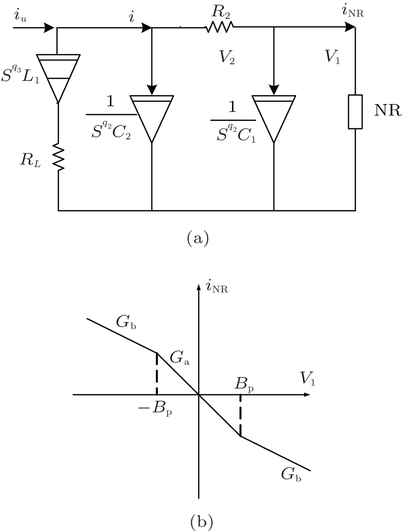 | Fig. 1. (a) Diagram of fractional order Chua’ s circuit. (b) Voltage current characteristic of NR. |
Let x = V1/BP, y = V2/BP, z = IL/BPG, α = C2/C1, β = C2/(L1G2), γ = C2R/(LG), m1 = Gb/G, m0 = Ga/G, τ = tG/C2, and u = Iu/BPG. Equations (11) and (12) can be rewritten as

and

Equation (14) can be rewritten as
For simplification, we set x(t) = x1 (t), y(t) = x2(t), z(t) = x3 (t). Equation (13) can then be written as

where A, B, and C are the system matrix, the input matrix, and the constant matrix, respectively. More specially,

Therefore, from the controllability theorem of a fractional linear system, we can obtain the following results. 1) When x(t) ≤ − 1 or x(t) ≥ 1, if and only if α (m1 + 1) ≠ γ + 2, the fractional Chua’ s circuit is controllable, otherwise the fractional Chua’ s circuit is uncontrollable. 2) When − 1 < x(t) < 1, if and only if α (m0 − 2m1 − 1) ≠ 2 + γ , the fractional Chua’ s circuit is controllable, otherwise the fractional Chua’ s circuit is uncontrollable.
In order to verify the controllability of the fractional Chua’ s circuit when α (m1 + 1) ≠ γ + 2 and α (m0 − 2m1 − 1) ≠ 2 + γ , we set α = 10, β = 10, γ = 0.2, q1 = 0.98, q2 = 0.8, q3 = 0.94, m0 = − 1, and m1 = − 0.9. The initial values of the system (x(0), y(0), z(0)) is (− 2, 1, − 1). We set the input u(t) as 5, 25, and 45 to study the controlling effect of the input u(t) on the system. The numerical simulations with different controllers u(t) are presented in Fig. 2.
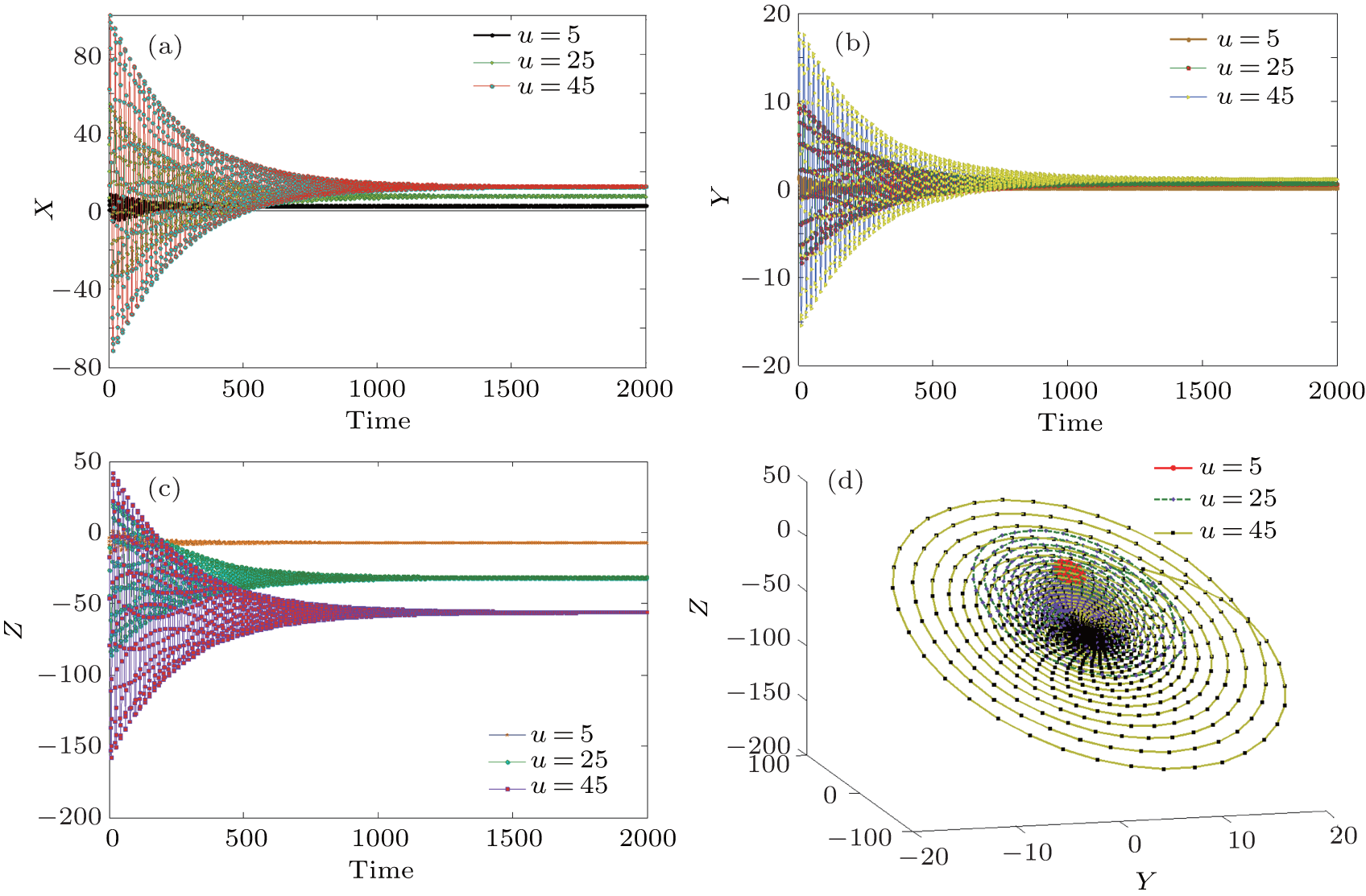 | Fig. 2. The response of system state with different controllers u(t): (a)– (c) time waveforms of state variables X, Y, and Z; (d) phase orbit of state variables X, Y, and Z. |
Figures 2(a)– 2(c) are the time waveforms of state variables X, Y, and Z, respectively. Figure 2(d) is the phase orbit of state variables X, Y, and Z. From Fig. 2(a), we know that the state variable X can be driven from initial state − 2 to different finial states 2, 8, and 12, respectively, by changing the input u(t). For different inputs u(t), as shown in Fig. 2(b), the state variable Y can also be driven from initial state 1 to different finial states 0.1, 0.5, and 1.1, respectively. Similarly, the state variable Z can be driven from initial state − 1 to different finial states − 8, − 30, and − 55, respectively. More specially, Figure 2(d) reveals the trajectories of state variables X, Y, and Z under the variations of the input u(t).
From the above analyses, we can easily obtain different final states by changing the controller u(t), which perfectly shows the controllability of the fractional order Chua’ s circuit system.
In this paper, we extend the conventional controllability theorem to the fractional domain by using strictly mathematical analysis and proof. Since Chua’ s circuit is a typical representative of nonlinear circuits, we study the controllability of the fractional order Chua’ s circuit in detail using the presented theorem. Numerical simulations and theoretical analysis are both presented, which are in agreement with each other.
We have proved that the Kalman rank condition is equivalent between the fractional order systems and the integer order systems. In addition, the controllable condition is applicative for arbitrary order. This is the foundation of research on the fractional order circuit with arbitrary structure. In the future, we will study this question and further develop the controllability theory of the fractional order circuit.
| 1 |
|
| 2 |
|
| 3 |
|
| 4 |
|
| 5 |
|
| 6 |
|
| 7 |
|
| 8 |
|
| 9 |
|
| 10 |
|
| 11 |
|
| 12 |
|
| 13 |
|
| 14 |
|
| 15 |
|
| 16 |
|
| 17 |
|
| 18 |
|
| 19 |
|
| 20 |
|
| 21 |
|
| 22 |
|
| 23 |
|
| 24 |
|
| 25 |
|
| 26 |
|
| 27 |
|
| 28 |
|
| 29 |
|
| 30 |
|
| 31 |
|
| 32 |
|
| 33 |
|
| 34 |
|
| 35 |
|
| 36 |
|