The interaction between matter and laser fields is an essential problem of quantum optics.^[1] Generally, laser fields are considered as monochromatic and they provide a coherent radiation field for studying laser– matter interactions.^{[2– 5]} Most laser theories and experiments demonstrate that the amplitude and phase of laser fields fluctuate with time.^[6] The fluctuation of the phase can be thought as the photon emission from atoms with random phase.^[1] The phase diffusion model is a widely accepted way to describe the phase fluctuation of a field.^{[6– 9]} In the phase diffusion model, the phase fluctuation is described by a Wiener– Lé vy stochastic process. The amplitude fluctuations of the field can be described by Markovian stochastic processes.^[10] Several groups have studied the effects of the fluctuations of the laser field on some optical properties, such as transition saturation, ^{[6, 11– 17]} resonance fluorescence, ^[6] ac Stark splitting, ^[7] optical susceptibility, ^[18] etc.

In this paper, we consider the V-type three-level systems interaction in an external field with fluctuating phase and amplitude. The density matrix operator is employed to describe the system. The density matrix satisfies the well-known optical Bloch equations (including random variables). When the random variables satisfy the Markovian stochastic processes with δ correlated Gaussian noise, the optical Bloch equations can be dealt as Langevin equations.^[6] Employing the techniques of multiplicative stochastic processes, one can obtain the averaged optical Bloch equations, and then the generating functions. We study the stochastic resonance phenomenon of the emission intensity I and Mandel' s Q parameter with respect to the pure dephasing constant γ _p via generating functions. The pure dephasing constant γ _p is caused by the fluctuating phase. The amplitude fluctuation of the field can make the Rabi oscillation decrease quickly, which will also make the systems lose their coherence quickly. On the other hand, the fluctuation of the amplitude can provide a new interference method via the pure amplitude fluctuation field driving strength (𝓦 ₂₃), which could help us to use the orthogonal system to obtain the phenomena which have just occurred in parallel system. In the pure amplitude fluctuation field, the emission intensity I also shows saturation phenomenon.

We consider V-type three-level systems driven by an external field. The V-type three-level systems are composed with a ground state| 1〉 and two degenerate excited states: | 2〉 and | 3〉 . The transition between the ground state | 1〉 , and the excited states | 2〉 and | 3〉 means that the electric dipole transition is allowed, and the corresponding electric dipoles are μ ₁₂ and μ ₁₃. The direct transition between the two excited states | 2〉 and | 3〉 is electric-transition-forbidden, which means that the electric dipole is μ ₂₃ = 0. In the dipole approximation, the Hamiltonian can be written as

where | n〉 and | m〉 are the eigen-states of the system, ω _n is the eigen-frequency of the eigen-state | n〉 , μ _nm is the electric dipole moment between states | n〉 and | m〉 , and we assume the permanent electric dipole moments μ _nn = 0, (n = 1, 2, 3), and μ _nm = μ _mn, (n, m = 1, 2, 3). E(t), the external field, can be expressed as

where 𝑒 _f, 𝓔 (t), ω _L, and φ (t) are the polarization, amplitude, angular frequency, and phase of the external field, respectively.

The density matrix ρ (t) of the system satisfies the Liouville– von Neumann equation^[19]

where 𝓛 ρ (t) is the damping term, which can be split into two parts 𝓛 ρ = 𝓛 ^{+ Γ} ρ + 𝓛 ^(r)ρ , ^[20]𝓛 ^{+ Γ} ρ represents the system emitting photon processes, and 𝓛 ^(r)ρ is the rest part. The generating function can be defined as, where ρ ^(k) is the density matrix of the system where it has emitted k photons, and s is the auxiliary coefficient for counting photons. The generating function 𝓖 (s, t) satisfies^[20]

In the rotating wave approximation (RWA), the generating functions can be written as

where Γ ₂ and Γ ₃ are the spontaneous emission rates of the eigen-states | 2〉 and | 3〉 , respectively, γ ₂₃ is the coherent damping rate, and Δ = ω _L – ω ₂₁ is the detuning frequency, and

The generating functions  (5)can be dealt with as Langevian equations when the fluctuation 𝓔 (t)e^{– i φ (t)} is Markovian stochastic process. Most of laser theories and experiments demonstrate that the Markovian stochastic process is a good approximation for the fluctuations of the field.^[6] For the Langevin equations

with F_ij(t) being δ -correlated Gaussian noise

after using the techniques of the multiplicative stochastic processes, ^[6] the mean values can be expressed as follows:

In this subsection we assume that the amplitude 𝓔 (t) = 𝓔 ₀ is time-independent and that the derivative of the phase with respect to time is a δ -correlated Gaussian random process,

and the initial phase φ ₀ shows uniform distribution between 0 and 2π , γ _p is the dephasing constant. By introducing the following variables

, and , and using the techniques of the multiplicative stochastic processes, one can obtain the mean values as follows:

where Ω _nm = – μ _nm· 𝑒 _f𝓔 ₀/ħ are the Rabi frequencies.

In this subsection, we assume that the phase φ (t) is time-independent, we choose φ (t) = 0, and the amplitude 𝓔 (t) can be expressed as

where 〈 𝓔 〉 is the average amplitude, and δ 𝓔 (t) is the δ -correlated Gaussian noise,

where𝓓 is the correlation constant of the amplitude.

By substituting Eq.  (12) into the generating functions  (5), and using the techniques of the multiplicative stochastic processes, the mean value of the generating functions can be expressed as

where Ω _nm = – μ _nm· 𝑒 _f〈 𝓔 〉 /ħ are the average Rabi frequencies, 𝓦 ₁₂ = (μ ₁₂· 𝑒 _f)²𝓓 /(2ħ ²), 𝓦 ₁₃ = (μ ₁₃· 𝑒 _f)²𝓓 /(2ħ ²), and 𝓦 ₂₃ = (μ ₁₂· 𝑒 _f)(μ ₁₃· 𝑒 _f)𝓓 /(2ħ ²) are the non-coherent pumping/damping rates.

One can then obtain the working generating function as^{[21– 23]}

where x_nm = g_nm is the phase fluctuation and x_nm = 𝓖 _nm is the amplitude fluctuation.

The factorial moments 〈 N_r 〉 of emission photons can be calculated as

The emission intensity I and Mandel' s Q parameter can be calculated as follows:^{[21– 23]}

In this paper, we consider two kinds of V-type three-level systems; that is, the parallel (μ ₁₂∥ μ ₁₃) and the orthogonal (μ ₁₂⊥ μ ₁₃) interactions with the fluctuating field. In our calculation, the spontaneous emission rates are Γ ₂ = Γ ₃ = Γ , is the parallel system, γ ₂₃ = 0 is the orthogonal system, and the splitting energy ω ₃₂ = 5Γ is between the two excited states.

The phase fluctuation of the laser field gives frequency fluctuationto the laser angular frequency ω _L. One can define an effective angular frequency as . According to the phase diffusion model, is the zero mean value and δ represents the correlated Gaussian stochastic process. For a fixed time t′ , the distribution of is the Gaussian distribution and the width of the distribution is . As γ _p increases, the width of the distribution increases. The distribution of the effective angular frequency ῶ _L is also Gaussianian, and the width of the distribution is determinated by γ _p. The distribution of the effective angular frequency ῶ _L makes the line shape of the single molecule show an extra broaden phenomenon.^[24] Figure  1 demonstrates the emission intensity I and Mandel' s Q parameter as a function of γ _p. The Rabi frequency is Ω ₁₂ = Ω ₁₃ = Γ and the detuning frequency is Δ = 2.5Γ . The red lines represent the emission intensity I and Mandel' s Q parameter of the parallel system and the black lines represent that of the orthogonal system. The emission intensity I shows the stochastic resonance with respect to the pure dephasing constant γ _p. For a fixed detuning frequency Δ , there exists an optimal pure dephasing constant γ _p, which makes the emission intensity reach its maximum value. Mandel' s Q parameter demonstrates that the emission photons show anti-bunching behavior at the phase fluctuation.

Fig.  1.

	Figure Option ViewDownloadNew Window
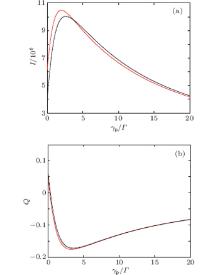
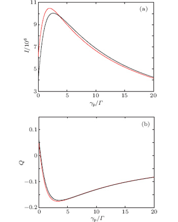	Fig.  1. The emission intensity I (a) and Mandel' s Q parameter versus γ p (b). The red lines represent the emission intensity and Mandel' s Q parameter of the parallel system and the black lines represent that of the orthogonal system. The Rabi frequencies are Ω 12 = Ω 13 = Γ , the detuning frequency is Δ = 2.5Γ , the calculation time is Γ t = 105, and the system is in the ground state.

Figure  2 demonstrates the Rabi oscillation of the emission intensity I and Mandel' s Q parameter. The red lines represent the emission intensity I and Mandel' s Q parameter of the parallel system and the black lines represent that of the orthogonal system. The solid lines correspond to 𝓦 ₁₂ = 𝓦 ₁₃ = 0, the dashed lines correspond to 𝓦 ₁₂ = 𝓦 ₁₃ = 𝓦 ₂₃ = Γ , and the detuning frequency is Δ = 2.5Γ . In this condition, the parallel V-type three-level system will show coherence population trapping for long time limit, but for a short time the emission intensity I and Mandel' s Q parameter will also show the well-known Rabi oscillations. The amplitude fluctuation of the field makes the amplitude of the Rabi oscillation decrease faster. In this condition, the three-level systems can be considered as an effective two-level system, the excited state is, and then the Rabi oscillation can be expressed as cos(Ω t) if no damping terms exist. The amplitude fluctuating of the field makes the Rabi frequency Ω become Ω ′ = Ω + δ Ω . Then, the Rabi oscillation could become 〈 cos (Ω ′ t) 〉 = exp(– γ _dt) cos(Ω t), with 〈 δ Ω ² 〉 = 2γ _d, and δ Ω is the δ -correlated Gaussian noise. This means that the fluctuation of the amplitude gives an external damping constant to the Rabi oscillation, which could make the Rabi oscillation more invisible.

Fig.  2.

Figure Option ViewDownloadNew Window

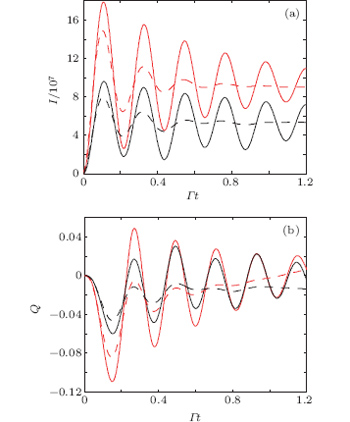Fig.  2. The emission intensity I (a) and Mandel' s Q parameter (b) versus time t. The red lines represent the emission intensity and Mandel' s Q parameter of the parallel system and the black lines represent that of the orthogonal system. The solid lines correspond to the 𝓦 12 = 𝓦 13 = 0 and the dashed lines correspond the 𝓦 12 = 𝓦 13 = 𝓦 23 = Γ . The average Rabi frequencies are Ω 12 = Ω 13 = 20Γ , the detuning frequency is Δ = 2.5Γ , and the system is in the ground state.

Figure  3 demonstrates the quantum beats of the three-level systems driven by a pure amplitude fluctuating field (which means 〈 𝓔 (t)〉 = 0, the corresponding average Rabi frequencies Ω _ij = 0). The red lines represent the emission intensity I and Mandel' s Q parameter of the parallel system, the blue lines represent that of the orthogonal system, and the green lines are the reference lines which indicate that no quantum beats have occurred. The red lines are oscillating with time t, which represent the population exchange between two excited states | 2〉 , and | 3〉 via γ ₂₃ and 𝓦 ₂₃. The system jumps from its excited state | 3〉 (| 2〉 ) into the ground state | 1〉 , and emits a photon. The photon is immediately absorbed by the system and the system has been excited into the other excited states | 2〉 (| 3〉 ) from its ground state | 1〉 .^{[21, 25]} The blue lines show the population exchange between the two excited states | 2〉 and | 3〉 via 𝓦 ₂₃. From Eq.  (14), one can know that 𝓦 ₂₃ appears in the same position as γ ₂₃, which means that 𝓦 ₂₃ plays the role of γ ₂₃. The amplitude fluctuation of the external field provides a new interference way between the two excited states | 2〉 and | 3〉 in the orthogonal V-type three-level system.

Fig.  3.

Figure Option ViewDownloadNew Window

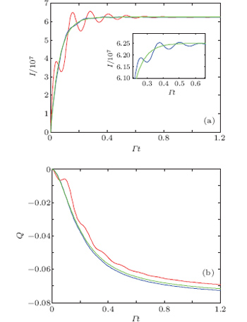Fig.  3. The emission intensity I (a) and the Mandel' s Q parameter (b) versus time t. The red lines represent the emission intensity and the Mandel' s Q parameter of the parallel system, the blue lines represent that of the orthogonal system. The average Rabi frequencies Ω 12 = Ω 13 = 0, 𝓦 12 = 𝓦 13 = 𝓦 23 = Γ , the green lines represent the reference lines corresponding to 𝓦 23 = 0, which represent the case with no quantum beats have occurred and the system is in the ground state.

Figure  4 demonstrates the emission intensity I (a) and Mandel' s Q parameter (b) versus θ , which is the angle between the electric dipole μ ₁₂ and the polarization vector e_f. The red lines represent the emission intensity I and Mandel' s Q parameter of the parallel system and the black lines represent that of the orthogonal system. The average Rabi frequencies are Ω _ij = 0 (the pure amplitude fluctuating field). For the parallel system, the emission intensity I reaches its maximum value at θ = nπ , (n = 0, 1, 2, … ), which corresponds to the direction of the field paralleling or anti-paralleling to the electric dipole μ ₁₂ and μ ₁₃. The emission intensity I also shows saturation phenomenon at θ = nπ as the curve of I is deviated from the sine function, which is clearly demonstrated by Mandel' s Q parameter. The minimum value of Mandel' s Q parameter is at θ ∼ nπ ± 0.3π , (n = 0, 1, 2, … ), which corresponds to the critical driving field strength for the saturation. The emission intensity I and Mandel' s Q parameter of the orthogonal system are oscillating with θ , when I reaches its minimum and Q reaches its maximum. In this condition, the system can be considered as an effective two-level system and the corresponding electric dipole μ is along direction θ = π /4.

Fig.  4.

	Figure Option ViewDownloadNew Window
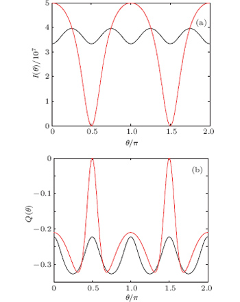	Fig.  4. The emission intensity I (a) and Mandel' s Q parameter (b) versus θ . The red lines represent the emission intensity and Mandel' s Q parameter of the parallel system, and the black lines represent that of the orthogonal system. The average Rabi frequencies are Ω 12 = Ω 13 = 0, 𝓦 12 = 𝓦 13 = 𝓦 23 = Γ , the calculation time is Γ t = 105, and the system is in the ground state.

The phase fluctuation of the field shows an extra broadening phenomenon to the line shape of the system and the emission intensity I shows stochastic resonance with respect to the pure dephasing constant γ _p. The amplitude fluctuation of the field gives an extra damping constant to the Rabi oscillation and the damping constant is proportional to 〈 δ 𝓔 (t)²〉 . The emission intensity I and Mandel' s Q parameter demonstrate the quantum beats phenomenon as the system is driven by the pure amplitude fluctuation field (〈 𝓔 〉 = 0). The 𝓦 ₂₃ plays the same role as γ ₂₃ in the system, the orthogonal system also shows the quantum beats phenomenon via 𝓦 ₂₃. This means that one can simulate a parallel system via a driven orthogonal system. The emission intensity I and Mandel' s Q demonstrate the saturation phenomenon, even in a driving field with pure amplitude fluctuation.