
Onsager principle as a tool for approximation
[Doi Masao† ]
]
]
|
|


Corresponding author. E-mail: masao.doi.octa.pc@gmail.com
Onsager principle is the variational principle proposed by Onsager in his celebrated paper on the reciprocal relation. The principle has been shown to be useful in deriving many evolution equations in soft matter physics. Here the principle is shown to be useful in solving such equations approximately. Two examples are discussed: the diffusion dynamics and gel dynamics. Both examples show that the present method is novel and gives new results which capture the essential dynamics in the system.
Onsager principle is the variational principle proposed by Onsager in his celebrated paper on the reciprocal relation.[1, 2] The principle has been shown to be useful in deriving many time evolution equations in soft matter physics, [3, 4] such as the Chan– Hilliard equations in phase separation, [5] kinetic equations in gel dynamics, [6] Ericksen– Leslie equation in liquid crystals, [7] etc. In this paper, the principle is shown to be useful in obtaining approximate solutions for such equations.
The base of the Onsager principle is that if there are certain set of slow variables, which will be detailed later, their evolution equations are derived by the variational principle proposed by Onsager.[1, 2, 4] If we have a complete set of slow variables, we can derive their evolution equations as it has been done previously.[3, 4] If the slow variables are not complete, the evolution equations will not be accurate, but we expect that they will give a good approximation as long as they represent the characteristic slow dynamics of the system. In the following, it will be shown that this is actually the case. This will be demonstrated by two examples, the diffusion dynamics and the gel dynamics. These examples will demonstrate the novelity and usefulness of the present method.
The Onsager principle is an extension of Rayleigh’ s principle of the least energy dissipation in Stokesian hydrodynamics.[8] In fact, for isothermal system, the principle can be stated in the same form as the minimum energy dissipation principle. Here the Onsager principle is explained by taking a problem in hydrodynamics.
Consider many particles moving in a viscous fluid. Let x = (x1, x2, … , xf) be the generalized coordinates specifying the state of the particles, where f is the degree of freedom of the system; for a rigid particle, f is 6, and xi stands for the position and orientation of the particle. Let U(x) be the potential energy of the system: U(x) can be the gravitational energy or the interaction energy between the particles. The potential force conjugate to xi is given by

Let ẋ i be the variable representing the time derivative of xi, i.e., the generalized velocity. If a particle moves in a Newtonian fluid, the fluid exerts a frictional force on the particle. In the limit of small Reynolds number, the frictional force is written as a linear function of ẋ i:[8]

The coefficients ζ ij are called friction coefficients: they are functions of x, and can be calculated by Stokesian hydrodynamics.
The friction coefficients ζ ij satisfy the reciprocal relation and positive definiteness, i.e.,

The reciprocal relation allows us to write the frictional force as follows:

where Φ is defined by

The function Φ is called the dissipation function. It is equal to half of the work done to the fluid per unit time, Φ = − (1/2)Σ i FHiẋ i.
Since the Reynolds number is assumed to be negligibly small in Stokesian hydrodynamics, the frictional force must be balanced with the potential force. This gives the following equation
Let (ζ − 1)ij be the inverse of the matrix ζ ij, then equation (6) gives a time evolution equation for xi
The above set of equations [Eqs. (5) and (6)] can be regarded as a special case of the Lagrangian mechanics in dissipative systems. It has been proposed that the Euler Lagrange equation in dissipative system can be written as[9]

where K is the kinetic energy of the system. If the kinetic energy term is ignored, equation (8) reduces to Eq. (6). Such a reduction is justified in the “ overdamped regime” where the frictional force is much larger than the inertia term. The dynamics we discuss here is valid in such regime.
Onsager noticed that many kinetic equations which describe time evolution of non-equilibrium systems are written in the form of Eq. (6) or Eq. (7). He then proved that as long as the equation is written in this form, the coefficients (ζ − 1)ij or ζ ij are symmetric. This remarkable relation, called Onsager’ s reciprocal relation, is the base of the Onsager’ s variational principle.
With the reciprocal relation (3), the time evolution equation (6) can be cast into a variational principle. We define Rayleighian

where Φ is defined by Eq. (5) and 

The force balance equation (6) is equivalent to the condition ∂ R/∂ ẋ i = 0, i.e., the evolution of xi is determined by the condition that R be minimum with respect to ẋ i. This is the Onsager principle.[1, 2, 4]
The base of the variational principle is the reciprocity and the positive definiteness of ζ ij (Eq. (3)). In Stokesian hydrodynamics, these properties can be proven directly based on the Stokes equation for the fluid velocity. The remarkable thing here is that the reciprocity and the positive definiteness of ζ ij is not limited to hydrodynamic systems. It is based on the existence of slow variables. The slow variables are the variables the relaxation time of which is distinctively longer than that of other variables. In such a case, it can be shown that the total force acting on slow variables when they are changing with rate ẋ = (ẋ 1, ẋ 2, … ) is written as (see Ref. [4])

where U now stands for the free energy of the system in which the other variables (fast variables) are at local equilibrium for given values of slow variables. Equation (11) is a result of a perturbation calculation for the distribution function of fast variables:[4] the first term represents the average force when the slow variables are fixed, and the second term represents the first order perturbation when the slow variables are changing at rate ẋ = (ẋ 1, ẋ 2, … ). The condition that the total force Fi, tot must be zero when the system is evolving spontaneously gives the evolution equation (6).
The reciprocal relation ζ ij = ζ ji can be directly proven by the microscopic expression for ζ ij (i.e., the fluctuation dissipation theorem). Therefore the Onsager principle can be justified if there are certain set of slow variables.
The Onsager principle tells us how to derive evolution equations of non-equilibrium systems for given slow variables. In applying the principle to practical problems, the crucial step is to choose slow variables. Therefore how to choose the slow variables is an important problem, and it is discussed here briefly.
The slow variables are the state variables which specifies the non-equilibrium state. They have to satisfy the following conditions.
(i) If the slow variables (x1, … , xf) at time t is given, their value at the next time step t + Δ t must be uniquely determined: the set of variables (x1, … , xf) must be the complete set of variables to describe the dynamics of the system. In other words, there should be no hidden variables which creates the memory effect in the dynamics.
(ii) The other fast variables not included in the slow variables must be close to the local equilibrium state specified by the slow variables. If the slow variables are fixed at x, the free energy of the system is written as a function of x as U(x). If the slow variables are changed slowly at rate ẋ , the distribution of first variables is slightly perturbed from the local equilibrium state, creating a force FHi which is linear in ẋ .
In the hydrodynamic systems, the slow variables are the variables specifying the configuration of the particles, and the fast variables are the rest variables specifying the configuration of fluid molecules. Given x, i.e., given the configuration of particles at time t, the configuration at time t + Δ t is uniquely determined. Notice that this is true only for Newtonian fluid. If the fluid is a complex fluid such as liquid crystals or polymer solutions, other variables (such as director field, or the polymer configuration tensors) are needed to predict the particle configuration at the next time step.
The evolution equation given by the Onsager principle has always the form of Eq. (7). This form of the evolution equation actually includes quite a large class of equations such as the diffusion equation, phase separation kinetic equation, gel dynamic equations, etc., as it has been demonstrated in Refs. [3] and [4].
To illustrate the usage of the Onsager principle, let us first consider the problem of diffusion. Consider the one-dimensional diffusion, and let n(x; t) be the number density of particles at position x and time t. Notice that the slow variable in the present problem is given by a continuous function n(x; t). The free energy of the system is written as a functional of n(x). In dilute solutions, this is given by

where kBT is the Boltzmann constant multiplied by temperature. Our objective is to find out the time evolution of n(x). The term 

On the other hand, it is not easy to write down the dissipation function Φ as a functional of ṅ (x). However, if we introduce the flux velocity v(x) of particles, which is connected to ṅ (x) by the conservation equation

the dissipation function is easily written down

where ζ is the friction constant of a particle.
The conservation equation (14) indicates that we are considering the situation that n(x) can change only by diffusion. In general n(x) may change by chemical reaction, but equation (14) states that such a process is not considered here. The flux velocity v(x) is needed to represent such physical constraint.Using Eqs. (13), (14) and performing the integral by parts, we can write 

Hence the Rayleighian is given by

The minimum of this is given by

Equations (14) and (18) give the diffusion equation

In the previous section, we regarded n(x; t) as a slow variable and derived the evolution equation using the Onsager principle. Let us now use the same principle to solve the diffusion equation approximately.
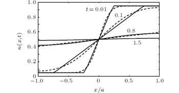
Consider that the particles are confined by two walls located at x = − a and x = a and that at time t = 0, the concentration profile is a step-function

where sign(x) is equal to 1 for x > 0 and − 1 for x < 0. Time evolution of n(x; t) is easily obtained by solving the diffusion equation (19) for this initial condition. The result is

Here we solve the problem by a different method using the Onsager principle.
As time goes on, the slope of n(x; t) at x = 0 decreases, and eventually becomes zero. Therefore we expect that the solution can be approximated as nx; t = n0 + α (t)x in the range where the slope of n(x; t) is non-zero;

where x1 = n1/α . We regard α (t) as a slow variable, and derive the evolution equation for it using the Onsager principle. Clearly, α (t) is not the slowest variable in the system. (The slowest variable is the eigenfunction corresponding to the smallest eigenvalue of the diffusion operator.) However since α (t) is a good parameter representating the non-equilibrium state of the system, we expect that it will also be a good slow variable representing the dynamics. Let us now see whether this expectation works or not.
Given the functional form of n(x, t), the velocity v(x, t) is obtained by the conservation equation (14):
Equation (23) is solved for v(x, t) with the boundary condition v(a, t) = 0

Substitution of Eq. (24) into Eq. (17) gives the following energy dissipation function
where 

where ζ eff is a function of α and is defined by

where ∊ = n1/n0. Likewise, 

with
Therefore the evolution equation for α becomes

For small α (t), equation (30) gives

with
The slope α (t) decreases exponentially with the relaxation time τ app = 2a2/5D = 0.4 a2/D. On the other hand, the exact solution of the diffusion equation indicates that the longest relaxation time of the current problem is τ exa = 4a2/(π 2D) = 0.405 a2/D. Therefore the approximate solution gives a reasonably accurate relaxation time.
The approximate relaxation time τ app is smaller than the exact relaxation time τ exa. This is always the case. It can be proven that the longest relaxation time obtained by the present approximate method is always smaller than that of exact solution.
An interesting feature of the present method is that it gives a good approximation even in short time scale. In short time t ≪ τ , equation (30) gives

where

Equation (33) gives

On the other hand, the slope of the exact solution at x = 0 is given by

The power law behavior of α (t) in short time agrees with that of the exact solution.
Figure 1 shows the comparison between the approximate solution and the exact solution. It is seen that our piece-wise linear solution is a good approximation of the exact solution over the entire regime of time scale. Notice that the present method of approximation gives a nonlinear evolution equation which describes the relaxation dynamics in both the power law regime α (t) ∝ t− 1/2 and the exponential regime α (t) ∝ e− t/τ .
Gel is a homogeneous mixture of elastic material and fluid. In a typical gel, a polymeric gel, the gel consists of cross-linked polymer and solvent. The cross-linked polymer forms a three-dimensional network and gives an elasticity to the gel.
The deformation of polymer network is coupled with the diffusion of solvent. For example, when a gel is compressed, solvent is expelled from the gel. Conversely, when solvent diffuses into a gel, the gel deforms. Equations describing such coupling has been derived with the use of the Onsager principle.[6] The slow variable here is the vector u(r, t) which represents the displacement of the point on the network located at r in a certain reference state. If the displacement is small, the free energy is given by the same form as the elastic energy of deformation

where K and G are material constants called osmotic bulk modulus and shear modulus respectively.
On the other hand, the energy dissipation is given by

where υ s stands for the velocity of the solvent, and ξ is the friction constant of polymer network per unit volume.
In constructing the Rayleighian, we have to take into account of the fact that gel behaves as an incompressible material (i.e., the volume change of a gel can occur by taking in (or out) solvent from (or to) surrounding solution. This constraint is expressed as

where ϕ is the volume fraction of polymer. Since we are considering the case of small deformation, we may assume ϕ to be constant.
The Rayleighian is thus constructed as


and

where

Equations (41) and (42) are the basic equations which describe the coupling of deformation and diffusion in a gel. Applications of these equations are discussed in Ref. [6].
If temperature of a gel is changed, the gel changes its volume by absorbing or expelling solvent. This swelling (or de-swelling) process is rather complex as it involves the coupling between solvent diffusion and network deformation. Analytical solution has been obtained only for special cases. Here we use the Onsager principle to obtain an approximate solution for a slab-shaped gel.
Consider a slab-shaped gel having edge length 2a, 2b, and 2c. We assume a ≥ b ≥ c for convenience of later discussion. We take the origin of the Cartesian coordinate at the center of the slab. Therefore a point in the gel is specified by (x, y, z), with − a < x < a, − b < y < b, and − c < z < c. We assume that displacement vector of each point is given by

and that the velocity of the solvent is given by

where ∊ α (t) and κ α (t) (α = x, y, z) are the variational parameters to be determined. Substituting Eqs. (44) and (45) into Eq. (38), the energy dissipation function is given by

where V = 8abc is the initial volume of the gel. The free energy of the gel is given by

where weq represents the volume change weq = Δ Veq/V when the gel gets the new equilibrium state. Hence the Rayleigian becomes
The last term in Eq. (48) represents the incompressible condition (39).
Straightforward calculation for the evolution equation derived from the Rayleighian (48) gives the following conclusions.
i)The gel swells isotropically:
where w(t) = Δ V(t)/V is the volume change at time t.
ii)The volume change is single exponential:
where ξ ̃ = ξ /(1 − ϕ ).
The first conclusion i) is surprizing. Since the diffusion takes place most quickly along the shortest path from the surface, one may expect that the equilibration of ∊ z takes place faster than ∊ y and ∊ x. However, equation (49) indicates that the equilibration takes place at the same speed in all directions, i.e., the gel swells keeping its aspect ratio constant. Though surprizing, such result has also been obtained by exact calculation for cylindrical gels. It has been shown that for a cylinder of large aspect ratio, the ratio between the axial length and the outer radius of the cylinder remains constant during the swelling process.[10] Therefore it is likely that gel generally swells keeping its shape almost the same as the original although there is no proof for this conjecture.
The second conclusion ii) is also surprizing. According to Eq. (50), the relaxation time depends on the osmotic bulk modulus K, but not on the shear modulus G. This is not correct in general. The relaxation time of a gel generally depends on both K and G. However, it is known that in the two limits of K ≫ G and K ≪ G, the longest relaxation time depends on K only. Indeed the longest relaxation time can be written as[11]

where ℓ is a certain length. The simple expression of Eq. (50) captures this surprizing feature of the swelling dynamics.
Equation (50) also indicates that the longest relaxation time is mainly determined by the length of the shortest edge, c, which is reasonable and in accordance with exact calculation for slabs.[4] Therefore, equation (50) captures all the essential physics involved in the swelling dynamics of gels. This again demonstrates that the Onsager principle gives quite a useful tool of approximation.
We have shown that the Onsager principle is useful in solving many problems in soft matter physics. It is useful in deriving time evolution equations, in both precise and approximate description. We have shown this by two examples. The first example of diffusion is quite simple, but it demonstrates a unique and interesting feature of the present method: the Onsager principle gives a nonlinear differential equation which represents the characteristic feature of the solution of the linear diffusion equation. The second example of gel swelling gives a simple, yet non-trivial result for the swelling dynamics.
The base of the Onsager principle is that there are certain set of slow variables. Many problems in soft matter have such structures, and can be handled by the Onsager principle. We will show this with more examples in future.
This work started while I was staying at Denmark Technical University supported by Otto Moensted Foundation to give a lecture course on soft matter physics. I thank Prof. Ole Hassager and Otto Moensted Foundation for giving me this opportunity which motivated the present work.
| 1 |
|
| 2 |
|
| 3 |
|
| 4 |
|
| 5 |
|
| 6 |
|
| 7 |
|
| 8 |
|
| 9 |
|
| 10 |
|
| 11 |
|