Recursion-transform approach to compute the resistance of a resistor network with an arbitrary boundary
[Tan Zhi-Zhong† ]
]
]
|
|


Corresponding author. E-mail: tanz@ntu.edu.cn, tanzzh@163.com
We consider a profound problem of two-point resistance in the resistor network with a null resistor edge and an arbitrary boundary, which has not been solved before because the Green’s function technique and the Laplacian matrix approach are invalid in this case. Looking for the exact solutions of resistance is important but difficult in the case of the arbitrary boundary since the boundary is a wall or trap which affects the behavior of a finite network. In this paper, we give a general resistance formula that is composed of a single summation by using the recursion-transform method. Meanwhile, several interesting results are derived by the general formula. Further, the current distribution is given explicitly as a byproduct of the method.
The computation of two-point resistances in networks is a classical problem in electric circuit theory and graph theory.[1– 5] Nowadays, research on the resistor network is expanded into the basic model in the field of science and engineering.[6– 20] A lot of abstract and complex scientific problems have been solved by modeling resistor networks[11– 20] since the German scientist Kirchhoff (1824– 1887) founded the node current law and the circuit voltage law in 1845. The previous research on resistor networks has focused on the infinite networks due to the poor technology, [3] and little attention has been paid to finite networks, even though the latter occur in real life. Looking for the exact solution of resistance between any two nodes in a resistor network in the finite case is important but difficult. The construction of, and research on, the models of resistor networks therefore are of significance in theory and application.
In 2000, Cserti[3] evaluated a two-point resistance of a resistor network by using the lattice Green’ s function which is confined to regular lattices of infinite size. In 2004, Wu[4] formulated a different approach and derived an expression for the two-point resistance in arbitrary finite and infinite lattices with a normative boundary (such as free, periodic boundary, etc.) in terms of the eigenvalues and eigenvectors of the Laplacian matrix. Laplacian analysis has also been extended to impedance networks after a slight modification of the formulation in Ref. [5], and recently it has been applied to a cobweb network.[8] However, the Laplacian approach cannot be applied to the matrix with arbitrary elements. The actual computation depends crucially on the geometry of the network and, for nonregular lattices such as a resistor network with arbitrary boundaries, it is incapable of solving the eigenvalue problem. However, the boundary condition is important because it is a real case occurring in real life. The boundary is a wall or trap which affects the behavior of a finite network.
Recently we[9, 10] proposed a new method to calculate the two-point resistance in a network. We used this method to compute the equivalent resistance, which relies on just one matrix along one direction, and expressed the exact resistance by single summation. Using the description in Refs. [9] and [10] we refer to this method as the recursion-transform approach (or the RT method). When just one boundary or a pair of opposite boundaries are arbitrary, the RT method is still valid for the computation of resistance. The RT method has been used to solve many problems of the resistor network. For example, in 2013 a cobweb model and a conjecture were proposed by us, [9, 10] soon afterwards a globe network was solved.[11] Almost at the same time, the cobweb conjecture was solved in Ref. [12]. Very recently a cobweb network with 2r boundary was solved.[13]
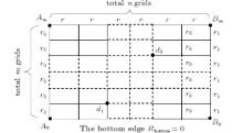
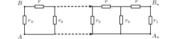
We consider an m× n resistor network with resistances r and r0 in the respective horizontal and vertical directions, except for the arbitrary right edge and the bottom boundary, as shown in Fig. 1. This paper focuses on the computation of the two-point resistance between any two nodes in the resistor network with an arbitrary boundary, which has not been solved before because the Green’ s function technique and the Laplacian matrix approach are invalid in this case.
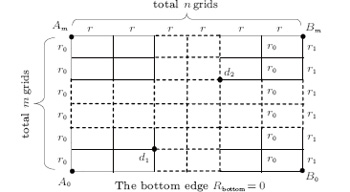 | Fig. 1. An m × n resistor network with arbitrary right boundary and null resistors at the bottom. The bonds in the horizontal and vertical directions are resistors r and r0, except for the bottom and right boundaries. |
The rest of this paper is organized as follows. In Section 2, we present several exact formulae of the resistance between any two nodes in a resistor network with an arbitrary boundary. In Section 3, we prove the equivalent resistance by the recursion-transform method, and test the formula by an example. In Section 4 a summary and discussion of the method and results are presented.
In order to facilitate the computation of the equivalent resistance of a resistor network, we define variables 

where 


We consider an m × n resistor network as shown in Fig. 1. Assume that A0 is the origin of the rectangular coordinate system, then the left edge will act as a Y axis and the bottom edge as an X axis. Denoting nodes of the network by coordinate {x, y}, the equivalent resistance between any two nodes d1 (x1, y1) and d2 (x2, y2) in the m × n resistor network can be written as
In particular, we have the following special cases.
Cases 2.1 When n → ∞ , x1, x2 → ∞ with x1 − x2 being finite, we have
Case 2.2 When m, n → ∞ , but y1, y2, and x1 − x2 are finite, we have
where Sk = sin(ykθ ), and 
Case 2.3 When m, n → ∞ but x1 − x2 and y1 − y2 are finite, we have
Case 2.4 When d1 = (x1, 0) is at bottom edge and d2 = (x2, m) is at top edge, we have
Case 2.5 When d1 and d2 are both at the left edge at d1(0, y1) and d2 (0, y2), we have
Case 2.6 When d1 and d2 are both on the left boundary, and m, n → ∞ , we have
Case 2.7 When d1= (0, y1) is at the left edge and d2= (n, y2) is at the right edge, we have
Case 2.8 When h1 = 0, we have
The general formula (4) and the above eight cases are given for the first time. From expression (4) we can deduce a lot of simple results because the r1 is an arbitrary resistor and m, n are two arbitrary natural numbers.
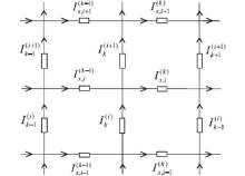
Assume that the electric current J is constant and goes from the input d1 to the output d2, as shown in Fig. 1. Denote the currents in all segments of the network as shown in Fig. 2. The resulting currents passing through all m + 1 row horizontal resistors with the same resistance of r are 
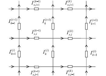 | Fig. 2. Sub-network of resistors with marked parameters and directions of the currents. |
We use Ohm’ s law to compute the resistance Rm× n (d1, d2). All of the nodes on the bottom boundary can be uniformly called O because the resistances of the bottom resistors are all zero. The voltages between two nodes O and d1, and two nodes O and d2 are, respectively,
Using Ohm’ s law, we have
How to solve the current parameters 

Using Kirchhoff’ s law (KCL and KVL) to analyze the resistor network, the node current equations and the mesh voltage equations can be achieved from Fig. 2. We focus on the four rectangular meshes and nine nodes, and give the relations in the absence of an injected current,
where h = r/r0 is a ratio of two resistance. Equation (14) can be written in a matrix form after considering the input and output current

where Ik and Hx are, respectively, m × 1 column matrix, and reads

where []T denotes matrix transpose, and (Hk)i is the element of Hx with the injection of current J being at d1 (x1, y1) and the exit of current J being at d2 (x2, y2). And
Equations (15)– (18) form the matrix equation model of the m× n resistor network.
How to solve the matrix equation (15) is the key to the problem. In this section we consider the solution of Eq. (15) in the absence of an injected current, namely: J = 0. Here we rebuild a new difference equation to solve Eq. (15) indirectly. To realize the idea, first we multiply Eq. (15) from the left-hand side by m × m undetermined square matrix Pm. Thus we have

We conduct the transformation of diagonal matrix by the following identity:

where Tm = diag(t1, t2, … , tm) is a diagonal matrix. Solving Eq. (20) we obtain

where θ i = (2i − 1)π /(2m + 1), and
A simple calculation shows that, the new matrix Pm is invertible, with the following inverse matrix:
By Eqs. (19) and (20) we define

where Xm is an m × 1 column matrix, and reads

Using Eqs. (19) and (24), we obtain the equation

where (read ζ x1, i as ζ 1, i, ζ x2 , i as ζ 2, i)
Equation (26) is much simpler than Eq. (15) because it is a linear equation that is easily derived. Suppose that λ i,
Next, we consider the solution of Eq. (26) when the injection of current J is at d1 (x1, y1) and the exit of current J is at d2 (x2, y2). We therefore need to consider the piecewise solution of Eq. (26) and obtain


where 
We consider the boundary conditions of the left and right edges in the network. By applying Kirchoff’ s laws (KCL and KVL) to a single mesh adjacent to each of the left and right boundaries, we obtain three matrix equations to model the boundary currents, that is,

where Em is an m-dimensional unit matrix, and Am is given by Eq. (18).
Conducting the same matrix transformation as in Eq. (19), and applying Pm to Eqs. (34) and (35) on the left-hand sides, we have

The above equations and transformations are proposals for the computation of the equivalent resistance. Next we derive two solutions of 

Substituting Eq. (36) into Eq. (29) to eliminate 

where 

where

is used. Using Eq. (37) to eliminate 

where we define bi = ti + (h1 − 2).
To obtain the initial conditions 


where ti = 2(1 + h) − 2hcos θ i is given by Eq. (21), and bi = ti + (h1 − 2) appearing in Eq. (40). Solving Eq. (41), we obtain after some algebra and reduction the solution of 
where 
Substituting Eq. (42) into Eq. (38) with k = x1 yields
Equation (13) obviously shows the key currents
where k = 0, 1, 2, … , n. Taking k = x1, we therefore achieve the following equation:
where the identity 
Similarly, taking k = x2 in Eq. (45), we also obtain
Substituting Eqs. (46) and (47) into Eq. (13) we obtain
Finally, we obtain the main result (4) by further substituting
In this section we will prove several special results that were proposed in Section 1 by formula (4).
Case 3.6.1 when n → ∞ with m being finite, by Eqs. (1) and (2) we obtain
where a = (λ i + h1 − 1) and 
Similarly, we obtain
Substituting Eqs. (50) and (51) into Eq. (4), we obtain Eq. (5) after having used 
Case 3.6.2 In order to prove Eqs. (6) and (7), we need to refer an integral theory, as follows.
If θ k = (2k − 1)π /(2m + 1), we have Δ θ k = θ k + 1 − θ k = 2π /(2m + 1). In the limit of m → ∞ , we have

which is an identity valid for any function g(θ k). Equation (52) is prepared to prove Eqs. (6) and (7) in the following.
When m, n → ∞ , but y1, y2, and x1 − x2 are finite, making use of Eqs. (5) and (52) we immediately obtain Eq. (6).
Case 3.6.3 According to the identity transform of a trigonometric function, we have
When m → ∞ and y1, y2 → ∞ , we must transform

where p, q ≪ m are integers, and (p − q) = (y1 − y2) are finite. As θ i = (2i − 1)π /(2m + 1), we have

Thus
By Eqs. (5) and (53) we obtain
Thus equation (7) is proved.
Case 3.6.4 When d1 is at the bottom edge (x1 , 0) and d2 is at the top edge d2 (x2, m), since d1 is on the null resistor edge, we have x1 = x2, thus

and
Since 
Case 3.6.5 When d1 and d2 are both on the left edge, we have x1 = x2 = 0. Since 


So, by Eq. (4) we obtain Eq. (9).
Case 3.6.6 When m, n → ∞ with x1 = x2 = 0, taking limit
Substituting Eq. (55) into Eq. (9), and using Eqs. (52) and (53), we obtain Eq. (10).
Case 3.6.7 When d1 is at the left edge (0, y1) and d2 is at the right edge (n, y2), we have x1 = 0 and x2 = n. Thus 
Substituting Eq. (56) into Eq. (4), we obtain Eq. (11).
Case 3.6.8 When h1 = 0, we have 
Because the main formulae are too complicated to understand, we will verify their correctness by an example.
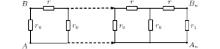
When m = 1, figure 1 degrades into a 1× n resistor network with an arbitrary right boundary, as shown in Fig. 3. When we compute the resistance between nodes A and B, then we have y1 = 0, y2 = 1. Thus by Eq. (2) we have θ i = θ 1 = π /3, and 
 | Fig. 3. The 1 × n resistor network with arbitrary right boundary. |
From Eq. (9) we obtain the resistance
where h = r/r0, h1 = r1/r0, and 
Formula (59) is fully consistent with the result in Ref. [9]. In particular, when n = 1, from Eq. (59) we have
Obviously, formula (60) is completely accordant with the actual circuit. In fact, our results are bound to be perfect since all of the processes of algebra and reduction are strict and self-consistent.
For the explicit computation of two-point resistance, Cserti[3] evaluated the two-point resistance using the lattice Green’ s function and restricted his study to regular lattices of infinite size. In 2004, Wu[4] established a theorem to compute the equivalent resistance between two nodes in a resistor network using the Laplacian approach, and he restricted his study to a regular boundary. The arbitrary boundary is a wall or trap which affects the behavior of a finite network. When the network is of finite size and with arbitrary boundary, Green’ s function technique and the Laplacian matrix approach are both invalid.
In the present article, we solve a complicated problem of a resistor network with an arbitrary boundary by the RT method. Our results are given in the form of a single summation. This method splits the derivation into three parts. The first part is to create a recursion relation (expressed by matrix) between the current distributions on three successive vertical lines. The second part is to diagonalize the matrix relation to produce a recurrence relation involving only variables on the same transverse line. The third part is to derive a recursion relation between the current distributions on the boundary. Basically, the method reduces the problem from two dimensions to one dimension.
The RT method can be extended to impedance networks because it is formulated on Ohm’ s law and this is also applicable to impedances. In addition, the grid elements r and r0 can be either resistors or impedances, we can therefore study an m × n complex impedance network, such as

Based on the plural analysis, the formula of the equivalent impedances of the m × n RLC network with an arbitrary boundary can be obtained.
| 1 |
|
| 2 |
|
| 3 |
|
| 4 |
|
| 5 |
|
| 6 |
|
| 7 |
|
| 8 |
|
| 9 |
|
| 10 |
|
| 11 |
|
| 12 |
|
| 13 |
|
| 14 |
|
| 15 |
|
| 16 |
|
| 17 |
|
| 18 |
|
| 19 |
|
| 20 |
|