Unified treatment of the bound states of the Schiöberg and the Eckart potentials using Feynman path integral approach
[Diaf A.† ]
]
]
|
|


*Project supported by CNEPRU (Grant No. D03920130021).
Corresponding author. E-mail: s_ahmed_diaf@yahoo.fr
We obtain analytical expressions for the energy eigenvalues of both the Schiöberg and Eckart potentials using an approximation of the centrifugal term. In order to determine the ℓ-states solutions, we use the Feynman path integral approach to quantum mechanics. We show that by performing nonlinear space–time transformations in the radial path integral, we can derive a transformation formula that relates the original path integral to the Green function of a new quantum solvable system. The explicit expression of bound state energy is obtained and the associated eigenfunctions are given in terms of hypergeometric functions. We show that the Eckart potential can be derived from the Schiöberg potential. The obtained results are compared to those produced by other methods and are found to be consistent.
The search for exact solutions of the radial Schrö dinger equation constitutes a very useful research area and is of general interest. Many efforts have been made to study the scattering and bound states of relativistic and non-relativistic cases with some physical potential models.[1– 4] It is well known that exact solutions for the s-state (angular momentum ℓ = 0) cannot be generalized to the case of the state with arbitrary angular momentum. In this case, the radial Schrö dinger equation as well as relativistic Dirac and Klein– Gordon equations are solved either numerically[5] or by approximation methods.[6– 12]
Among the potentials under consideration, we mention the class of exponential-type potentials, such as the Morse, Woods– Saxon, Hulthé n, and Manning– Rosen potentials. For these potentials the Schrö dinger equation admits an exact solution for ℓ = 0.[13– 15]
In the case of nonzero angular momentum states, accurate eigenvalues are reached by using an appropriate approximation scheme for the centrifugal term. Different methods have been used in this sense, such as the standard method, [16] the asymptotic iteration method, [17] supersymmetric quantum mechanics, [18] and the exact quantization rule method.[8]
In this paper, we study another exponential-type potential, namely an attractive hyperbolical potential of the form

where D, α , and σ 0 are positive parameters.
Studying the energy eigenvalues of diatomic molecules was first suggested by Schiö berg in 1986[19] as an alternative to the Morse potential. He suggested that the potential function (1) is more accurate than the Morse potential function in fitting the experimental Rydberg– Klein– Rees (RKR) potential energy curves and the rotational– vibrating levels for some diatomic molecules. Wang et al.[20] showed that a simple version of the Schiö berg empirical potential function and the well-known Manning– Rosen potential energy function are the same empirical function, and the Wei potential energy function and the Tietz potential energy functions are also the same solvable empirical function.[21]
Using the dissociation energy and the equilibrium bond length for a diatomic molecule as explicit parameters, Wang et al.[22] generated improved expressions for two versions of the Schiö berg potential energy function. Both versions of the Schiö berg potential function are Rosen– Morse and Manning– Rosen potential functions. By choosing the experimental values of the dissociation energy, equilibrium bond length, and equilibrium harmonic vibrational frequency as inputs, they calculated the average deviations of energies calculated with the potential model from the experimental data for five diatomic molecules and found that none of the six three-parameter empirical potential energy functions is superior to the other potentials in fitting the experimental data for all of the molecules examined.
The solutions of the Schrö dinger equation for the Schiö berg potential have been obtained for the s-wave case.[23] Motivated by the success of the approximate bound state solutions of the Feynman propagator with the Manning– Rosen and Rosen– Morse potentials, [24, 25] we attempt here to solve the general ℓ -wave propagator of the Schiö berg potential by using an improved approximation scheme of the centrifugal term that was proposed by Ikhdair et al.[26] The Eckart potential, which can be related to the Schiö berg potential by a change of parameters, is also treated. This is used in physics[27] as well as in chemical physics.[28, 29] We recall that the Feynman Path Integrals formalism only applies to the s-wave and we are faced with difficulties for nonzero ℓ -states similar to the ones encountered with the Schrö dinger equation.
The organization of this paper is as follows. In Section 2, we look for the most relevant approximation scheme of the centrifugal barrier to be used in the formulation of the path integral for the Schiö berg potential. In Section 3, using the Duru– Kleinert method, we determine the ℓ -wave eigenvalues for the Schiö berg potential. In Section 4, we study the Eckart potential. In Section 5 we present and discuss our results for both potentials. Our conclusions are summarized in Section 6.
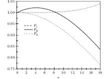
To deal with the centrifugal term some authors have used the approximation proposed by Greene and Aldrich, [11] which provides analytical results for arbitrary ℓ -wave bound states, scattering states of the Schrö dinger equation, and relativistic wave equations for different forms of exponential potentials.[16, 30, 31] In this approximation scheme, here labeled as F1, the centrifugal term is replaced by

As expected, this schematic approximation is more relevant when α is weaker. Other approximations have been proposed. For instance, Qiang[32] has suggested:

which we label as F2. A third scheme is due to Ikhdair in Ref. [26], which is labeled as F3

where the parameter C0 = 0.0823058167837972 is a shift determined by the expansion procedures. This value of C0 is an approximation. Indeed, the exact value of C0 is 1/12, as reported in Ref. [33]. This has been obtained using a power series decomposition (see Eq. (6) of Ref. [34]). For bound state solutions of the Schrö dinger equation with the Manning– Rosen potential and the Eckart potential, the numerical experiments showed that the analytical results obtained by employing the improved Greene– Aldrich approximation scheme are in better agreement with those obtained by using the numerical integration approach than the analytical results obtained by using the original Greene– Aldrich approximation scheme to deal with the centrifugal term.[35, 36]
Moreover, in order to compare the degree of validity of the three approximations, we display in Fig. 1 the graphs of the three expressions. This clearly shows that the approximation F3 is most suitable for the low values of α that are considered in this work. Consequently, this approximation F3 will be used throughout the present study.
 | Fig. 1. The plot of r2Fi, i = 1, 2, 3, with α = 0.05. |
In spherical coordinates, the time-sliced representation of the Feynman propagator takes the form[37]
Pℓ (cos θ ) denotes the Legendre polynomials with θ ≡ (r″ , r′ ) and

with

Here, Δ rj = rj – rj– 1, ɛ = tj – tj– 1, t′ = t0, and t″ = tN, and

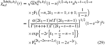
To solve Eq. (6) for nonzero angular momentum states, we apply the approximation F3 (included in Sj via ɛ Veff in Eq. (7)). Therefore, equation (7) becomes 
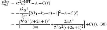
In a more compact form, it reads
where

In the following, we study the potential (9) in the framework of the Duru– Kleinert method.[38] The basic idea for solving this path integral problem is to find an appropriate space– time transformation to reformulate the path integral in terms of a well-known and already solved problem. This requires a relationship between the radial kernel of the Schiö berg potential and the radial kernel of a solvable quantum system.
The path integral for the potential (9) is
A convenient way to derive the corresponding transformation formula is to use the energy-dependent Green function G of the propagator Kℓ . By carrying out the point canonical transformation and the time transformation, [39]

we obtain the following Fourier transform formula

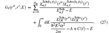
In Eq. (13) the Green function reads

where
and
The functions f′ , f″ , and f′ ″ denote the successive derivatives of f with respect to the variable q.
In our case, we choose
so as to obtain
Note that the transformation (17) leads to the following expression of the potential (9)

Collecting all these terms, we have

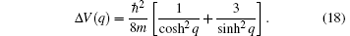
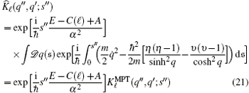
By substituting Eqs. (18) and (20) into Eq. (15), the effective potential Veff is now expressed in terms of the modified Pö schl– Teller (MPT) potential and the propagator expression becomes
with
and 

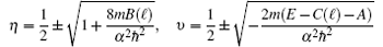
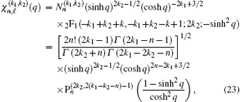
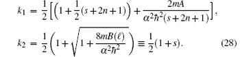
Here, we use the following notations:[43, 44] 2s = η (η − 1), – 2c = υ (υ − 1), where c ≤ 1/8, s ≥ − 1/8. The numbers k1, k2 are defined in terms of c and s as 

The upper limit Nm denotes the maximal number of states with 0, 1, ..., n ≤ Nm < k1 – k2 – 1/2. The signs, in the definition of k1, k2, depend on the boundary conditions for q → 0 and q → ∞ , respectively.
The propagator 
where 


where k = k1 – k2 – n. The corresponding eigenvalues are given by

Note that equation (23) has the appropriate Dirichlet conditions at q = 0 and q infinite when

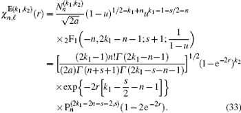
In the next section, we use the wave functions (23) and eigenvalues (25) of the modified Pö schl– Teller propagator to derive those corresponding to the Schiö berg potential.
Calculating 
By substituting Eq. (22) into Eq. (21), we get

Integrating Eq. (26) over the pseudo-time parameters s″ , the Green function G, equation (14), becomes
Following Refs. [24] and [39], the values of k1, k2, satisfying the appropriate boundary conditions for r → 0 and r → ∞ , are, respectively,
Substituting these values of k1, k2 in Eqs. (23) and (25), and introducing 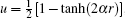
The energy spectrum is obtained from the poles of the Green function, Eq. (27), namely
We note that, in Eqs. (29) and (30), the angular momentum is present through the variable B, Eq. (10) and in the equations for k1, k2, and s, Eq. (28).
As mentioned above, we also consider the Eckart potential
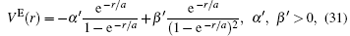
which is often used in chemical physics. The Eckart potential has been investigated, especially by Dong, [45] Zhang et al.[46] by means of the Nikiforov Uvarov (N.U.) method, [26] and Stanek, [47] who has used an improved approximation scheme to the centrifugal term. Here, the Eckart potential is combined with the approximation F3, to derive the corresponding path integral.
It should be noted that the Eckart potential reduces to the Schiö berg potential by setting α ′ = 4Dσ 0, 
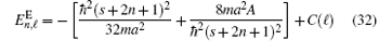
and
The parameters appearing in Eqs. (32) and (33) have been defined in Eqs. (10) and (28) and depend on ℓ .
Energies calculated by using the path integral method that is described above are reported in the following tables. The energy eigenvalues En′ , ℓ have been calculated for principal quantum numbers n′ = n+ ℓ + 1 and various angular quantum number ℓ , as in Ref. [47]. Two different values of the parameter σ 0 and a set of parameters α are considered. The present results for the Schiö berg potential Eq. (30) are displayed in Tables 1 and 2, and compared to the values given by Ikhdair and Sever, [26] who used the N.U. method with the same approximation of the barrier. All of the results are checked against the numerical data of Lucha et al., [5] who calculated the energies by using MATHEMATICA. The method of Ref. [5] gives the harmonic oscillator energies with a precision of 10− 5. We found that our calculated energy eigenvalues are improved as compared to the values of Ikhdair and Sever[26] and closer to the numerical results of Lucha et al.[5] At higher values of α both approaches are of similar quality. The relative error between our calculations and the numerical results is of about 2 × 10− 4 for all values of ℓ .
| Table 1. Eigenvalues – En′ , ℓ of the Schiö berg potential in atomic units (ħ = m = 1) with D = 10 and σ 0 = 0.1. |
| Table 2. Eigenvalues – En′ , ℓ of the Schiö berg potential in atomic units (ħ = m = 1) with D = 10 and σ 0 = 0.2. |
For the Eckart potential, the results, Eq. (32) are displayed in Table 3 and 4, where a comparison is made with the calculations of Stanek, [47] who analytically solved the Schrö dinger equation, but using another approach for the centrifugal barrier. All of the results are compared to the numerical data.[5] Our results are almost indistinguishable from the numerical ones.[5] Nevertheless, except in a few cases, we get results closer to the numerical estimates compared to the method of Stanek.[47] This is due to our choice of the centrifugal barrier.
| Table 3. Eigenvalues – En′ , ℓ of the Eckart potential in atomic units (ħ = m = 1) with α ′ = 1/a and β ′ = 0.0001. |
| Table 4. Eigenvalues – En′ , ℓ of the Eckart potential in atomic units (ħ = m = 1) with α ′ = 1/a and β ′ = 5 × 10– 5. |
In this paper, path integral formalism was used to solve two exponential-type potentials. We have calculated the energy levels of the Feynman kernel with the Schiö berg and the Eckart potentials for angular momentum ℓ ≠ 0, approximating the centrifugal term. First, we have shown that the most appropriate approximation scheme of the centrifugal barrier for this type of potential is the one given by Eq. (4). Then, the Duru– Kleinert transformation allows us to convert a nonsolvable propagator to another solvable one, for which the energy spectrum and the wave functions are known. This, allows us to determine analytically the energy spectrum of the starting potential.
Our results show that the obtained eigenvalues are in very good agreement with those given by other approximate methods and turn out to be in good agreement with the numerical data. The quality of our results proves that we can provide analytical eigenenergies and corresponding eigensolutions of the spectrum of the potential because the treatment of the barrier allows a tractable calculation leading to analytical results.
When the barrier approximation is fixed, we note that the Feynman integral method gives results closer to a numerical method than solving the Schrö dinger equation via the N.U. method.
To conclude, our method is efficient in solving this type of potential. We intend in the near future to expand the path integral method to a more general form of potentials and relativistic cases.
I would like to thank Dr. R. J. Lombard for his careful reading of the manuscript. I expresses my thanks to the Theory Group of IPN Orsay for the kind hospitality afforded to me, and the University of Khemis Miliana for its financial support (CNEPRU: D03920130021).
| 1 |
|
| 2 |
|
| 3 |
|
| 4 |
|
| 5 |
|
| 6 |
|
| 7 |
|
| 8 |
|
| 9 |
|
| 10 |
|
| 11 |
|
| 12 |
|
| 13 |
|
| 14 |
|
| 15 |
|
| 16 |
|
| 17 |
|
| 18 |
|
| 19 |
|
| 20 |
|
| 21 |
|
| 22 |
|
| 23 |
|
| 24 |
|
| 25 |
|
| 26 |
|
| 27 |
|
| 28 |
|
| 29 |
|
| 30 |
|
| 31 |
|
| 32 |
|
| 33 |
|
| 34 |
|
| 35 |
|
| 36 |
|
| 37 |
|
| 38 |
|
| 39 |
|
| 40 |
|
| 41 |
|
| 42 |
|
| 43 |
|
| 44 |
|
| 45 |
|
| 46 |
|
| 47 |
|