
Response of a Duffing—Rayleigh system with a fractional derivative under Gaussian white noise excitation*
[Zhang Ran-Ran, Xu Wei† , Yang Gui-Dong, Han Qun]
, Yang Gui-Dong, Han Qun]
|
|


Corresponding author. E-mail: weixu@nwpu.edu.cn
Project supported by the National Natural Science Foundation of China (Grant Nos. 11172233, 11302170, and 11302171) and the Natural Science Foundation of Shaanxi Province, China (Grant Nos. 2014JQ1001).
In this paper, we consider the response analysis of a Duffing–Rayleigh system with fractional derivative under Gaussian white noise excitation. A stochastic averaging procedure for this system is developed by using the generalized harmonic functions. First, the system state is approximated by a diffusive Markov process. Then, the stationary probability densities are derived from the averaged Itô stochastic differential equation of the system. The accuracy of the analytical results is validated by the results from the Monte Carlo simulation of the original system. Moreover, the effects of different system parameters and noise intensity on the response of the system are also discussed.
The study of the dynamic response of a stochastic system first began in 1905, when Einstein analyzed the Brownian movement of pollen particles in water. Recently, the response of a nonlinear stochastic system has become a popular topic in theoretical research and engineering practice due to the fact that nonlinear and random phenomena exist widely in nature, society, and engineering.[1– 4]
In the last few decades, the fractional derivative has received considerable attention.[5, 6] It cannot be denied that the fractional derivative has been used in various scientific and technological fields, [7– 10] such as signal processing, system control, diffusion, edge detection, robotics, biomedicine, turbulence, and viscoelasticity. In particular, the dynamical behaviors of oscillators with fractional derivatives have been studied by many researchers using various methods, and the most of them have considered the deterministic case.[11– 16] However, the analyses of stochastic systems with a fractional derivative have been proven to be unfruitful. Spanos and Evangelatos[17] obtained the random response of a SDOF nonlinear system with fractional derivatives using time domain simulation and statistical linearization technique. Liu et al.[18] proposed a residue calculus method to study the response of an axially moving viscoelastic beam with random noise and fractional-order constitutive relation. Ye et al.[19] presented the Fourier transform technique to analyze the stochastic response of structures with a fractional derivative. Among the approximate procedures in the field of stochastic dynamics, the stochastic averaging method is one of the most powerful methods. Recently, Huang and Jin[20] studied the response of single-degree-of-freedom systems with fractional-derivative damping using the stochastic averaging method. The first passage and bifurcation of stochastic systems with fractional derivative were investigated by Chen and Zhu.[21, 22]
The Duffing– Rayleigh oscillator is a canonical example of a self-excited and nonlinear system, and the presence of a cubic term makes the analysis of the Duffing– Rayleigh oscillator more complicated.[23] It has diverse applications in physics, biology, engineering, and many other fields.[24] To our knowledge, there is no analysis of the response of a Duffing– Rayleigh system with a fractional derivative. This subject forms the primary objective of this paper. The rest of this paper is organized as follows. In Section 2, we introduce Duffing– Rayleigh system with a fractional derivative under Gaussian white noise excitation. Approximate stationary probability density is derived by using the stochastic averaging method in Section 3. In Section 4, the analytical solutions are verified by numerical simulations and the effects of different system parameters and noise intensity on the stationary probability density are discussed. Our conclusions are presented in Section 5.
Considering a Duffing– Rayleigh system with a fractional derivative under Gaussian white noise excitation, the corresponding differential equation of motion is in the form of

where β 1 and β 2 denote coefficients of linear and nonlinear dampings, respectively; 

The potential energy function is

By using generalized harmonic functions the generalized displacement and velocity can be assumed to be in the following form:[26]


where the instantaneous phase Θ (t) and instantaneous frequency Λ (A, Θ ) can be written as

in which

We then expand Λ (A, Θ ) into a Fourier series with respect to Θ as follows:

where

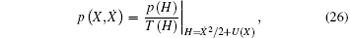
Integrating Eq. (8) with respect to Θ from 0 to 2π leads to the following approximate averaged frequency:

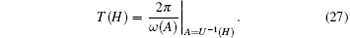
By substituting Eq. (4) into Eq. (1) and using the compatibility condition of Eq. (4), one obtains the stochastic differential equations of amplitude A and phase angle Γ as follows:


where


According to the Stratonovich– Khasminskii theorem, [27]A(t) converges weakly to a diffusive Markov process as ɛ → 0, even in a semi-infinite time interval. Thus, the limiting process can be described by the averaged Itô stochastic differential equation. Converting Eq. (11) into the Itô stochastic differential equation by adding the Wong– Zakai correction term leads to

where the drift and diffusion coefficients, respectively, are


In order to calculate the drift and diffusion coefficients more easily, the following approximate expression can be obtained by substituting Eq. (10) into Eq. (5):

Note that A and Γ vary slowly with time, and the following approximate relation can be obtained by using Eq. (15)

By using the above relation, the deterministic averaging of the term associated with fractional derivative on the right-hand side of Eq. (14a) can be simplified as follows:
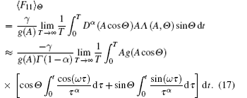
In order to simplify Eq. (17), the following integrals can be asymptotically expanded
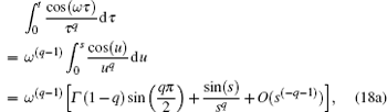
By substituting Eq. (18) into Eq. (17) and completing the averaging, equation (17) becomes
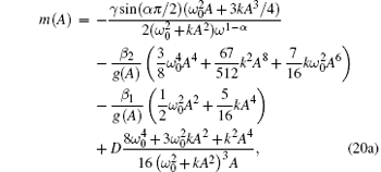
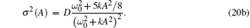
Finally, substituting Eq. (19) into Eq. (14a) and completing the averaging with respect to Θ yields the averaged drift and diffusion coefficients, as follows:
Based on the knowledge of the drift and diffusion coefficients, the Fokker– Planck– Kolmogorov (FPK) equation associated with Eq. (13) is in the form of

The boundary conditions of FPK equation depend on domain V. The boundary conditions with respect to A are


Under these boundary conditions, the stationary solution of the original system (1) can be obtained by solving Eq. (21). The result is
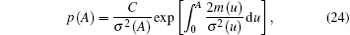
where C is a normalization constant.
The stationary probability density of the Hamilton function H = U (A) of the system (1) is in the following form
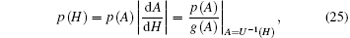
where U− 1 is the inverse function of U.
The joint stationary probability density of the generalized displacement and velocity is
where
The corresponding stationary probability densities of displacement X and velocity Ẋ , which mean the marginal distribution of Eq. (26), can be derived as


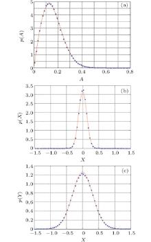
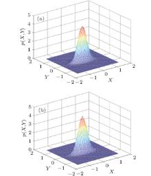
Based on the results in Eqs. (24)– (29), the stationary probability densities of amplitude, displacement, and velocity are shown in Fig. 1 when the system parameters are chosen to be α = 0.6, ω 0 = 2.5, k = 1.2, γ = 1.0, D = 0.06, β 1 = 0.05, and β 2 = − 0.05. The joint stationary probability densities of displacement and velocity are depicted in Fig. 2. It can be seen from Figs. 1(b) and 1(c) that the stationary response of the system is close to a Gaussian distribution and the peaks of the stationary probability densities of displacement and velocity appear at the constrained positions.
To assess the validity and accuracy of the proposed procedure, a predictor– corrector approach[28] is used for numerically simulating this system. Following this procedure, the results from numerical simulation with initial conditions x(0) = ẋ (0) = 0, time step h = 0.01 and 1.5 × 10⁶ samples for system (1) are also shown in Figs. 1 and 2. It can be observed that the analytical results from the stochastic averaging method are all in very good agreement with those from the Monte Carlo simulation of the original system.
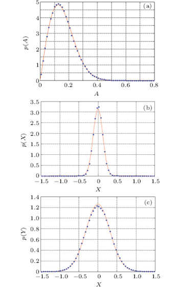 | Fig. 1. Stationary PDFs obtained analytically and numerically in the case of α = 0.6, ω 0 = 2.5, k = 1.2, γ = 1.0, D = 0.06, β 1 = 0.05, and β 2 = − 0.05: (a) PDF of amplitude A; (b) PDF of displacement X; (c) PDF of velocity Y = Ẋ . Here the lines denote the analytical results and the dots refer to the Monte Carlo results. |
 | Fig. 2. Joint PDFs of displacement X and velocity Y = Ẋ in the case of α = 0.6, ω 0 = 2.5, k = 1.2, γ = 1.0, D = 0.06, β 1 = 0.05, and β 2 = – 0.05: panel (a) shows the analytical result, and panel (b) refers to the Monte Carlo result. |
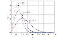
The response of system (1) is sensitive to the change in fractional order. Amplitude response curves of this system for different values of fractional order α in the case of ω 0 = 1.4, k = 4.0, γ = 3.0, D = 0.06, β 1 = 0.05, β 2 = − 0.05 are shown in Fig. 3. It can be found that the stationary probability densities of the amplitude move left and then the peak in a relatively small value as the fractional order α increases. From the view of probability theory, the higher peak of the stationary probability density means that there is a larger probability. Thus, this phenomenon can be explained as follows: as α increases, the system will move in a smaller range of amplitude with a high probability. It can be concluded that increasing α can reduce the degree of system response.
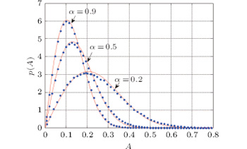 | Fig. 3. Stationary PDFs of amplitude A for different values of fractional order α in the case of ω 0 = 1.4, k = 4.0, γ = 3.0, D = 0.06, β 1 = 0.05, and β 2 = − 0.05. Here the lines represent the analytical results and the dots denote the Monte Carlo results. |
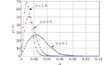
To check the effect of the coefficient of a fractional derivative on the response of the system, the stationary probability densities of amplitude for different coefficients of fractional derivative γ are depicted in Fig. 4. The amplitude response curves move left and their peaks are located at relatively small values as the coefficient of fractional derivative γ increases. Therefore, the higher coefficient of the fractional derivative leads to the lower response of the system.
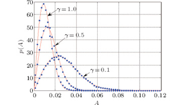 | Fig. 4. Stationary PDFs of amplitude A for different coefficients of fractional derivative γ in the case of α = 0.5, ω 0 = 1.0, k = 0.3, D = 6 × 10− 5, β 1 = 0.05, and β 2 = − 0.05. Here the lines represent the analytical results and the dots denote Monte Carlo results. |
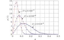
The noise intensity also has an obvious effect on the amplitude response curve. Figure 5 shows the stationary probability densities of amplitude, in which the results for different values of noise intensity D are compared. It can be seen that the increase of noise intensity leads to lower peaks and smoother curves. Similarly, the amplitude response curves for different values of natural frequency ω 0 are shown in Fig. 6.
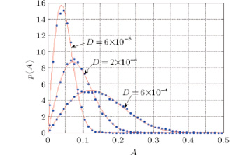 | Fig. 5. Stationary PDFs of amplitude A for different values of noise intensity D in the case of α = 0.5, ω 0 = 0.5, k = 1.0, γ = 0.1, β 1 = 0.05, and β 2 = − 0.05. Here the lines represent the analytical results and the dots denote Monte Carlo results. |
In Figs. 3– 6, the results obtained by using the stochastic averaging method agree well with the numerical simulation results of the original system. Moreover, the effects of the fractional order, the coefficient of fractional derivative, the noise intensity, and the natural frequency on the stationary probability density of amplitude are described clearly. This illustrates that research on the effects of different system parameters and noise intensity on the response of the system is very necessary.
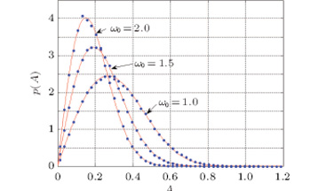 | Fig. 6. Stationary PDFs of amplitude A for different values of natural frequency ω 0 in the case of α = 0.6, k = 1.2, γ = 1.0, D = 0.06, β 1 = 0.05, and β 2 = − 0.05. Here the lines represent the analytical results and the dots denote the Monte Carlo results. |
In this paper, the response of Duffing– Rayleigh system with fractional derivative under Gaussian white noise excitation is studied by using the stochastic averaging method and the averaged FPK equation. A comparison between the analytical results and those from Monte Carlo simulations of the original system shows that the proposed procedure works well. The results show that the fractional order, the coefficient of fractional derivative, the noise intensity, and the natural frequency play important roles in the response of the system.
| 1 |
|
| 2 |
|
| 3 |
|
| 4 |
|
| 5 |
|
| 6 |
|
| 7 |
|
| 8 |
|
| 9 |
|
| 10 |
|
| 11 |
|
| 12 |
|
| 13 |
|
| 14 |
|
| 15 |
|
| 16 |
|
| 17 |
|
| 18 |
|
| 19 |
|
| 20 |
|
| 21 |
|
| 22 |
|
| 23 |
|
| 24 |
|
| 25 |
|
| 26 |
|
| 27 |
|
| 28 |
|