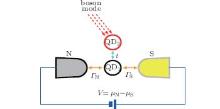
Fano-type interference arises when a discrete level is combined with a broad spectrum, giving rise to the asymmetric spectroscopic shapes.^[1] Such interferometric structures presently attract substantial interest in the study of electron propagation through disordered systems, ^[2] STM data for the Kondo-type impurities, ^[3] spectra of the heavy fermion compounds, ^[4] charge/spin transport through nanoscopic systems, ^[5] etc. In this work, we analyze the Fano-type lineshapes appearing in the subgap spectrum and the tunneling conductance of a double quantum-dot coupled between a normal (N) and superconducting (S) electrode, as shown in Fig. 1. In particular we examine how the bosonic bath (assumed as a monochromatic mode) combines with the proximity induced pairing and the strong electron interactions.

Fig. 1.

	Figure Option ViewDownloadNew Window
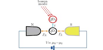	Fig. 1. Schematic view of the T-shape double quantum dot coupled between the metallic (N) and superconducting (S) electrodes, where the side-attached dot (QD2) is affected by a monochromatic boson mode (e.g., vibrons).

Under nonequilibrium conditions, charge can be transmitted between the external (N and S) electrodes either via the usual single particle tunneling (if applied voltage V is sufficiently large to break the electron pairs, | eV| ≥ Δ ) or by activating the anomalous Andreev channel. In the latter case, electrons from the normal electrode are converted into Cooper pairs in the superconducting lead, simultaneously reflecting the holes back to the metallic electrode. Differential conductance of such Andreev current is sensitive to both, the induced on-dot pairing and the electron correlations.^{[6– 10]} This issue has been studied theoretically for the single quantum dot^{[11– 17]} (see also other references cited therein) and the double quantum dot heterojunctions.^{[18– 25]}

Since nanoscopic objects (quantum dots, nanowires or molecules) are never entirely separated from their environment (e.g., photon^[26] or vibron^[27] quanta) therefore transport properties can reveal additional features originating from the constructive/destructive interference. In this work, we study the system (Fig. 1), where direct electron transport occurs via the central quantum dot (QD₁) and weak leakage to the side-coupled quantum dot (QD₂) contributes the interference effects. A similar mechanism has been investigated for the case with both normal electrodes^{[28, 29]} predicting the Fano-type resonances in the differential conductance, as has indeed been confirmed experimentally.^[30]

When quantum dots are hybridized with a superconducting reservoir, one expects interference patterns simultaneously in the particle and hole sectors, because of the induced on-dot pairing.^{[31, 32]} We have already analyzed such interferometric Fano resonances considering dephasing due to the external fermionic bath.^[33] In the present work, we extend such study taking into account the external bosonic mode.

In Section 2, we introduce the model and specify the characteristic energy scales. Next, we discuss formal aspects related to the approximations. In Section 4, we present signatures of the boson mode for the uncorrected quantum dots. Finally, in Section 5, we consider the correlation effects (including the Kondo regime). The appendix provides a simple phenomenological explanation of the Fano-type interferometric lineshapes of the heterojunctions consisting of two weakly coupled quantum dots.

The heterojunction shown in Fig. 1 can be described by the following microscopic Hamiltonian:

where Ĥ _N (Ĥ _S) refers to the normal (superconducting) charge reservoir, Ĥ _DQD describes the quantum dots together with a boson bath and the last term Ĥ _T corresponds to hybridization of the central QD₁ to external leads. We treat the conducting lead as a Fermi gas and describe the isotropic superconductor by the BCS Hamiltonian where denote the annihilation (creation) operators of mobile electrons with spin σ = ↑ or ↓ . The energies ξ _kβ = ε _kβ − μ _β are measured with respect to the chemical potentials μ _β , where μ _N − μ _S = eV.

We assume that an external bosonic bath directly affects only the side-attached quantum dot (QD₂). The Hamiltonian of the quantum dots and such a bosonic mode is given by

where are the annihilation (creation) operators of QD_{i= 1, 2} electrons, â ^{(† )} refer to the bosonic mode and . Usually ε _i denote the energy levels, λ is a coupling of the boson mode with QD₂, and ω ₀ is the bosonic energy. In what follows, we shall analyze the Fano-type interference originating from a weak coupling between both quantum dots (see the Appendix for details)

The model (1) can be generalized to more complex situations, for instance when both quantum dots are coupled to the external leads^{[16, 23]} and to the boson mode. For clarity, we focus on the case illustrated in Fig. 1, because it represents the simplest realization of the Fano-type lineshapes originating from the bosonic mode.

To study the electronic spectrum and the transport properties of the system (1), we introduce the matrix Green’ s function in the Nambu representation . In equilibrium conditions (μ _N= μ _S), the Green function depends only on time difference τ ₁− τ ₂ and its Fourier transform can be expressed as

where the bare Green functions g_i(ω ) are given by

The first part of the selfenergy comes from the hybridizations and the second term is due to the correlation effects.

3.1. Uncorrelated quantum dots

Let us start with the selfenergies of the uncorrelated quantum dots, that are solvable exactly. We can express them as

where g_β (k, ω ) denotes the Green functions of the leads. For the normal lead g_N(k, ω ) has a diagonal structure

and for the superconductor g_S(k, ω ) takes the BCS form

with the gaped quasiparticle energies and the coefficients , u_kv_k = Δ /2E_k.

In the wide band limit, one can introduce the constant hybridization functions Γ _β = 2π Σ _k| V_kβ | ²δ (ω − ξ _kβ ). Formally, we then obtain

with the auxiliary function^{[11, 12]}

Deep in a subgap regime (i.e., for energies | ω | ≪ Δ ), the expression (11) simplifies to a purely off-diagonal structure with the following static terms − Γ _S/2. One can hence interpret | − Γ _S/2| ≡ Δ _d1 as the pairing gap induced in the central quantum dot.^{[11— 14]}

3.2. Influence of a boson mode

To take into account the boson mode, we first determine the selfenergy of the side-attached quantum dot, neglecting the inter-dot coupling t. For convenience, we introduce the molecular Hamiltonian

and use the unitary transformation to eliminate the electron-boson coupling. Adopting the Lang– Firsov generating operator^[34]

one obtains^[35]

with the renormalized energy ε ̃ ₂ = ε ₂ − λ ²/ω ₀ and effective potential Ũ ₂ = U₂ − 2λ ²/ω ₀. Additionally, the operators

are dressed with the polaronic cloud

In absence of the interdot coupling, we can exactly determine the Green function G₂(ω ) using the identity

with T̂ _τ being the time ordering operator. The first part of Eq. (18) expresses invariance of the trace under the unitary transformation. The second line of Eq. (18) comes from the fact that statistical averaging with respect to the transformed Hamiltonian (15) is exactly equal to a product of the average with respect to the bosonic and the fermionic degrees of freedom. In particular, the polaronic propagator acquires the following standard form:^[35]

with the Bose– Einstein distribution N_p = [e^{β ω ₀} − 1]^{− 1}. Equation (19) can be used to compute the Fourier transform of the molecular Green function g_mol (ω ) ≡ lim_{t→ 0}G₂(ω ). Such a propagator has a diagonal structure with the following terms:^[36]

and g_{mol, 22}(ω ) = − [g_{mol, 11}(− ω )]*, where I_l denote the modified Bessel functions. At zero temperature the Green function (20) simplifies to

with the adiabacity parameter g= (λ /ω ₀)².

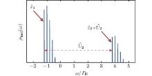
Effectively, the molecular spectral function ρ _mol(ω ) = − π ^{− 1}Img_{mol, 11}(ω + i0⁺) shows two groups of polaronic peaks (see Fig. 2). The lower polaronic branch starts at ε ̃ ₂ and the upper branch one is separated from it by Ũ ₂ (because the Coulomb potential U₂ is partly suppressed by the bipolaronic shift 2λ ²/ω ₀).^{[35, 36]} For the particular value g = 1, we observe about five peaks, but in the antiadiabatic regime (g ≫ 1), the number of boson peaks considerably increases.

Fig. 2.

	Figure Option ViewDownloadNew Window
	Fig. 2. The molecular spectral function obtained at zero temperature using the following set of parameters ε 2= − 1Γ N, U2= 5Γ N, ω 0= 0.2 Γ N, g=1, ε 1= 0.

In the succeeding sections, we treat the correlation effects (driven by the bosonic mode and the Coulomb repulsion U₂) within the following approximation:

which shall be reliable for the weak interdot coupling t.

3.3. Subgap transport

In a subgap regime | eV| < Δ , electrons are transmitted between the external electrodes practically only via the Andreev channel. Such anomalous current I_A(V) can be expressed by the Landauer-type formula^{[37– 39]}

where f(ω ) = [e^{ω /k_BT} + 1]^{− 1} is the Fermi– Dirac distribution. Andreev transmittance T_A(ω ) depends on the off-diagonal part of the Green function G₁(ω ) via^{[37– 39]}

Roughly speaking, equation (24) is a quantitative measure of the induced on-dot pairing and its optimal values coincide with the quasiparticle energies of the in-gap states. This transmittance T_A(ω ) also depends on the effects related to the quantum interference.^{[22, 24, 25, 33]}

Experimental measurements usually probe the differential conductance G_A(V) = ∂ I_A(V)/∂ V. We now discuss the spectrum and the tunneling conductance G_A(V) of the double quantum dot system: i) neglecting both Coulomb interactions U_i (Section 4) and ii) treating the electron-electron repulsion by suitable approximations (Section 5). Let us notice that T_A(− ω ) = T_A(ω ) implies the symmetric Andreev conductance G_A(− V) = G_A(V). This property comes from the fact that particle and hole states equally participate in the Andreev scattering.

In absence of both Coulomb interactions U_i we can determine the matrix Green functions G_i(ω ) using the Dyson equation (4) with the selfenergies Eqs. (6) and (7). We treat the influence of a boson mode through the local solution (22), assuming U₂ = 0. For small interdot coupling t ≪ Γ _β , the induced pairing affects mainly the low energy states of central dot (QD₁), therefore we focus on the case ε ₁ = 0, ε ₂ ≠ ε ₁. Figure 3 shows the equilibrium spectrum ρ _d1(ω ) obtained at zero temperature for g = λ /ω ₀ = 1 assuming the small boson energy ω ₀ < Δ . Such a case is interesting because the interferometric patterns appear in the subgap Andreev spectroscopy. Let us emphasize that the boson mode considered here is not related with the origin of superconductivity of the external lead. Such low energy boson mode could either represent the vibrational mode or the electromagnetic ac field. Such subgap vibration modes have indeed been reported experimentally for the carbon nanotubes suspended between external electrodes.^{[40, 41]} For the single quantum dot heterojunctions, this situation has been studied theoretically in Refs. [42]– [45].

Fig. 3.

	Figure Option ViewDownloadNew Window
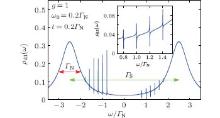
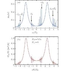
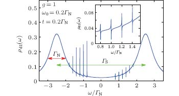	Fig. 3. The interferometric Fano-type lineshapes of the spectral function ρ d1(ω ) of QD1 obtained at T = 0 for the uncorrelated quantum dots (Ui = 0) using ε 1 = 0, ε 2 = 1Γ N, t = 0.2Γ N, Γ S = 5Γ N, and Δ = 10 Γ N.

We notice two Lorentzian peaks at the quasiparticle energies ± Γ _S/2 and two series of the Fano resonances. Such resonances appear at energies ± (ε ̃ ₂ + lω ₀) because of the particle– hole mixed excitations.^[31] The number of these interferometric features is sensitive to the adiabadicity parameter g. Only a few features appear in the adiabatic regime (g ≤ 1), whereas in the antiadiabatic limit, their number considerably increases. The Fano-type lineshapes also appear in the Andreev conductance (see Fig. 4). In comparison with the spectral function ρ _d1(ω ) the resonances are symmetrized for the reasons mentioned in the preceding section. Measurements of the subgap Andreev conductance would thus be able to detect such boson induced interferometric features.

Fig. 4.

	Figure Option ViewDownloadNew Window
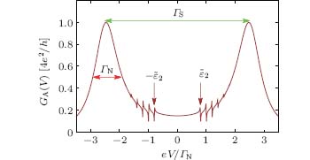	Fig. 4. The subgap Andreev conductance GA(V) obtained for the same parameters as in Fig. 3.

The in-gap quasiparticle peaks (often referred to as bound Andreev states) depend on the energy level ε ₁. In the case of a single quantum dot (i.e., for vanishing t), the spectral function ρ _d1(ω ) consists of two Lorentzians at ± E₁ (where broadened by Γ _N. Their spectral weights are given by the BCS factors (1 ± ε ₁/E₁)/2. This property also influences the interferometric features. Figure 5 shows the spectrum ρ _d1(ω ) for several values of ε ₁. When the energy level ε ₁ is more distant from the Fermi level, we observe a gradual redistribution of the quasiparticle spectral weights accompanied with suppression of the Fano resonances, especially at − (ε ̃ ₂ + lω ₀). The Andreev conductance G_A(V) is an even function of the voltage V; therefore, such particle-hole redistribution is not well pronounced, however suppression of the boson induced Fano lineshapes is noticeable.

Fig. 5.

	Figure Option ViewDownloadNew Window
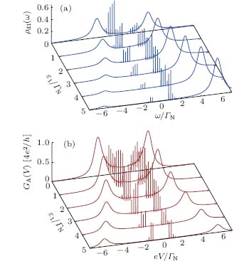	Fig. 5. Dependence of the spectral function ρ d1(ω ) (a) and the Andreev conductance GA(V) (b) on ε 1 (tunable by the gate voltage) for the same parameters as in Fig. 4.

In this last section, we discuss additional effects caused by the Coulomb repulsion U_i. Since electron transport occurs via the central quantum dot, we expect U₁ to play the most significant role. For completeness, we separately analyze the qualitative effects originating from both Coulomb potentials U_i.

5.1. U₁ = 0, U₂ ≠ 0

In order to study the influence of U₂, we simply use the approximate selfenergy (22), which is reliable in the case of weak interdot coupling. For stronger couplings t ≥ Γ _β , one should rather adopt the eigen-basis of the double quantum dot and consider higher-order correlation effects, like e.g., an indirect exchange interaction (between QD₂ and the metallic reservoir) which could induce the exotic Kondo effect.^[46] This interesting aspect, however, goes beyond the scope of the present study.

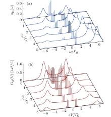
The upper panel of Fig. 6 illustrates the QD₁ spectrum ρ _d1(ω ) obtained at zero temperature for U₂ = 5Γ _N, U₁ = 0. As far as the spectrum of QD₂ is concerned, it still consists of two series of the bosonic peaks appearing around ε ̃ ₂ and near the Coulomb satellite ε ̃ ₂ + Ũ ₂, similar to what is shown Fig. 2, except a finite broadening of the peaks ∼ t²/D.

The Fano-type resonances appearing in ρ _d1(ω ) result from a combined effect of the interference (caused by the side attached quantum dot) and the proximity induced on-dot pairing. We can notice effectively four groups of such structures appearing near ± ε ̃ ₂ and ± (ε ̃ ₂ + Ũ ₂) due to the particle– hole mixing. These Fano structures also show up in the Andreev conductance G_A(ω ), though in a symmetrized way (bottom panel in Fig. 6).

Fig. 6.

	Figure Option ViewDownloadNew Window
	Fig. 6. Spectral function ρ d1(ω ) of the central quantum dot (a) and the differential Andreev conductance (b) obtained at zero temperature for ε 1 = 0, ε 2 = − 1Γ N, t = 0.2Γ N, g=1, ω 0 = 0.2Γ N, Δ = 10 Γ N, and U2 = 5Γ N.

5.2. U₁ ≠ 0, U₂ = 0

The potential U₁ has a qualitatively different influence on the transport properties than U₂. The central quantum dot is coupled between N and S leads therefore, it is affected by the on-dot pairing (promoted by Γ _S) and by the effective exchange interaction (due to finite Γ _N and U₁) leading to the Kondo effect. These phenomena are antagonistic. Their competition has been addressed so far by various groups using different many-body techniques (see e.g. Refs. [13] and [14] for a survey).

Here we analyze spectroscopic features of the system (Fig. 1) following our studies^{[47– 50]} based on the equation of motion technique (EOM).^[51] Such approximation proved to give satisfactory results for the single quantum dot heterojunctions.^{[7, 8]} We thus assume the correlation selfenergy in a diagonal form with

and . The other symbols appearing in Eq. (25) have the following meanings:^[51]Σ ₀(ω ) = ∑ _k| V_kN| ²/(ω − ξ kN) ≃ − i Γ _N/2 and

Equation (25) qualitatively captures both the Coulomb blockade and the Kondo effect, when ε ₁ < 0 < ε ₁ + U₁ and

Under such conditions, there appears a narrow Abrikosov-Suhl peak at ω = 0 whose broadening is scaled by k_BT_K. The EOM treatment is however not reliable in reproducing the low energy shape of this peak, that could be obtained from the numerical renormalization group calculations^{[11, 12, 32]} or other many-body methods.^{[52– 58]}

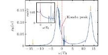
Let us briefly point out the characteristic properties of the Kondo regime. The spectral function of the central quantum dot (shown in Fig. 7) consists of four Lorentzians at energies of the Andreev bound states indicated by the arrows. Such quasiparticle subgap states are formed at and . We have chosen ε ₁ slightly below the Fermi level therefore, the quasipartice spectral weights are not symmetric. A part of the Lorentzians, we notice the narrow Kondo peak at the Fermi level. It is considerably reduced in comparison to the normal case Δ = 0 because of the competition between pairing and spin ordering.^{[47– 50]} Finally, we additionally recognize the Fano-type interference patterns at ± (ε ̃ ₂ + lω ₀).

Fig. 7.

	Figure Option ViewDownloadNew Window
	Fig. 7. Spectral function ρ d1(ω ) of QD1 obtained in the Kondo regime for kBT = 10− 3Γ N, ε 1 = − 2Γ N, U2 = 15Γ N, Γ S = 4Γ N, t = 0.2Γ N, ω 0 = 0.2Γ N, g=1, Δ ≫ Γ N. Vertical arrows indicate quasiparticle energies of the Andreev states (at ± E1 and their Coulomb satellites). We can notice the Kondo peak at ω = 0 coexisting with a number of the Fano-type resonances induced by the boson mode.

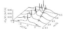
These features also show up in the subgap Andreev conductance. Figure 8 shows the maxima of G_A(V) at voltages corresponding to the quasiparticle energies of the Andreev bound states. Moreover, we notice the additional zero-bias enhancement due to the Kondo effect, which has indeed been observed experimentally.^{[7, 8]} On top of such behavior, there appear the Fano-type resonances. They can have a detrimental effect on the zero-bias Kondo feature when these interferometric features appear near the Fermi energy. We would like to emphasize also that this zero-bias anomaly is visible only when Γ _N ∼ Γ _S.^{[47– 50]}

Fig. 8.

	Figure Option ViewDownloadNew Window
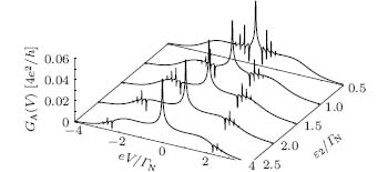	Fig. 8. Differential conductance of the Andreev current obtained in the Kondo regime for the same set of parameters as in Fig. 7 and for varying ε 2.

We have investigated the spectrum and Andreev conductance of the T-shape double quantum dot coupled between one metallic and another superconducting electrode. Focusing on the low energy (subgap) regime, we have studied the influence of a bosonic mode coupled to the side-attached quantum dot, converting its spectrum to the multilevel structure. Electrons tunneling through the central quantum dot are resonantly scattered (in a weak interdot coupling regime) by such multilevel “ molecule” , giving rise to the Fano-type interference patterns.

The effective spectrum of the central quantum dot and the differential conductance of the N– DQD– S junction reveal groups of equidistant bosonic resonances formed nearby ± (ε ̃ ₂ + lω ₀) and ± (ε ̃ ₂ + Ũ ₂ + lω ₀). Correlation effects due to the Coulomb potential U₁ do also significantly affect the spectroscopic properties. Spin of the central quantum dot is screened (at low temperatures) by itinerant electrons of the metallic lead provided that proximity induced pairing (promoting the BCS-type configurations) does not completely suppress it, see Ref. [32]. Quantum interference eventually obscures it whenever the Fano-type resonances appear close enough to the Kondo peak.

It would be worthwhile to extend our study to the case of stronger interdot coupling. Both quantum dots (as a whole) might then be characterized by new molecular eigen-states where the boson mode could manifest itself in a qualitatively different way, no longer resembling the Fano-type resonances. Under such circumstances, the Coulomb potential U₂ could play a very important role as U₁ via the indirect exchange interaction allowing for exotic realizations of the Kondo effect.^[46]