
Thermodynamic study of fluid in terms of equation of state containing physical parameters
Cite this Article
S. B. Khasare. Thermodynamic study of fluid in terms of equation of state containing physical parameters. Chinese Physics B, 2014, 24(1): 015101 
Permissions
Thermodynamic study of fluid in terms of equation of state containing physical parameters
Corresponding author. E-mail: shailendra.khasare@yahoo.com
Abstract
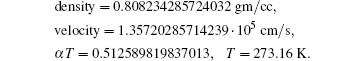
We introduce a simple condition for one mole fluid by considering the thermodynamics of molecules pointing towards the effective potential for the cluster. Efforts are made to estimate new physical parameter f in liquid state using the equation of state containing only two physical parameters such as the hard sphere diameter and binding energy. The temperature dependence of the structural properties and the thermodynamic behavior of the clusters are studied. Computations based on f predict the variation of numbers of particles at the contact point of the molecular cavity (radial distribution function). From the thermodynamic profile of the fluid, the model results are discussed in terms of the cavity due to the closed surface along with suitable energy. The present calculation is based upon the sample thermodynamic data for n-hexanol, such as the ultrasonic wave, density, volume expansion coefficient, and ratio of specific heat in the liquid state, and it is consistent with the thermodynamic relations containing physical parameters such as size and energy. Since the data is restricted to n-hexanol, we avoid giving the physical meaning of f, which is the key parameter studied in the present work.
Keyword:
51.30.+i; 05.70.Ce; equations of state; Lenard–Jones potential; hard-sphere potential
1. Introduction
In this paper, we use the equation of state (EOS), which was developed in earlier papers, [1– 7] to study the new parameter associated with clusters at different temperatures covering the liquid state only. The model is very simple, and demands one to study the role of the standard state. The main equation of state has already been published in the previous papers. The numerical results based on the equation of state and the associated results listed in tables are merely qualitative representations, however they lead to physical conclusions. The properties of hard sphere provide the theoretical backbone towards the equations of state for real fluids. The extended scaled particle theory[1– 3] is presently used to calculate thermodynamic measurable parameters. Since the equation of state is originally designed to capture the packing interactions in a fluid, it seems to be an ideal path for calculating thermodynamic measurable parameters through model parameters and vice versa. Two parameters are necessary for real fluids, the radius and the binding energy of the molecule. The author[4, 5] has used the equation of state for a strong repulsive potential together with a weak attractive potential.
The equation of state is a basic equation used to describe the relationship among pressure, volume, and temperature of a system. Perhaps the first one is the van der Waals equation of state, which can be used to describe thermodynamic properties for fluids qualitatively. The most popular model for the behavior of gases is the virial equation, in which the second and the higher-order virial coefficients have been investigated[8] extensively. Since the pioneering ideas[9] of Bernal and Scott[10] on the static packing models of hard spheres, assemblies of spherical particles interacting via a hard sphere potential have been studied quantitatively in order to model dense liquid and gas. Besides the hard sphere fluid, the Lennard– Jones fluid has also been investigated extensively. The equation of state is not only very important for studying the equilibrium thermodynamic properties, but also a basic equation used to predict the fluid surface properties such as surface tension and Tolman length, [11] and construct a Helmholtz energy functional for inhomogeneous fluids.[12] The density functional theory developed from the equation of state has been successfully applied to the pressure tensor[13] and the phase transition[14] for confined fluids.
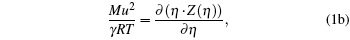
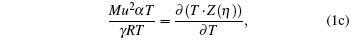
2. Mathematical model Z(η ) for real fluid
2.1. One parameter model
The following set of equations can be used for reproducing the thermodynamic profile:
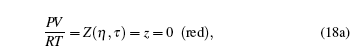
 |
 |
 |
 |
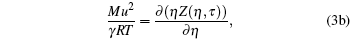
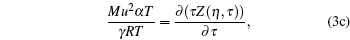
where two physical properties (R, γ ) along with the model parameter η can be evaluated for any real fluid by assuming any model fluid. It is observed that the above thermodynamic properties are highly sensitive to the choice of hard sphere (cavity) radii. Normally a real fluid can be represented by a minimum of two parameters such as the size of the molecule and its binding energy. Hence the equation of state containing a single parameter has limited success. A different size of cavity (model parameter) is required to reproduce a different thermodynamic property. Because the hard sphere model, which is used for real fluids, is not at all sufficient and significant to reproduce density, volume expansion coefficient, and velocity data simultaneously.
The physical significance of R is the work per degree per mole. It may be expressed in any set of units representing work or energy (such as joules), other units representing degrees of temperature (such as degrees Celsius or Fahrenheit), and any system of units designating a mole or a similar pure number that allows an equation of macroscopic mass and fundamental particle numbers in a system, such as the ideal gas. In order to take deviation or check the gas constant in a liquid state for any model equation, let R→ ζ .R, then the above set of equations becomes
 |
 |
 |
The above three equations are the basic equation of state and the partial derivatives with respect to temperature and volume. This set of equations can be used to determine (i) deviation parameter ζ for scaling thermodynamic variables such as pressure, volume, temperature, and gas constant; (ii) γ associated with the ratio of specific heat; (iii) model parameter η . Hence the solution set is a triplet (ζ , γ , η ). The present calculation shows that the ratio of specific heat does not have a logical domain [0 < γ ≤ 1.6667] corresponding to ζ = 1 (no deviation) and vice versa for an assumed model function Z, which naturally depends on η
2.2. Two parameters model
Hence it is necessary to use the equation of state, which contains a minimum of two model parameters (σ , ε ), and there should be one-to-one correspondence between model variables and thermodynamic variables, i.e., (σ , ε ) → (V, T),
 |
 |
 |
 |
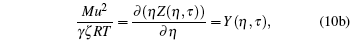
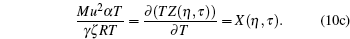
It is a simple observation that all thermodynamic potentials are primarily determined by any two thermodynamic variables such as volume and temperature. For a given EOS, introducing scaling parameter ζ for existing thermodynamic variables such as P, V, T or a constant such as R along with model parameters such as regular molecular cavity diameter σ and binding energy ε , then the above set of equations becomes
 |
 |
 |
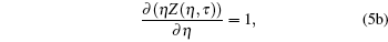
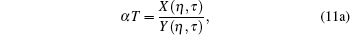
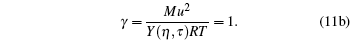
One can evaluate model variables (η , τ ) in terms of model parameters (σ , ε ). Hence the inter consistency demands a set of solutions in terms of unique triplet [ζ , η , τ ]. Here the model variable again depends on scaling parameter ζ , which means [η (ζ ), τ (ζ )] and [σ (ζ ) , ε (ζ )]. Hence we conclude that model variables (η , τ ) depend on ζ , which is to be decided by the set of three equations. If we accept the variation of ζ , which means that it has to be related to some measurable physical properties, then the gas constant is a universal constant only when η → 0, τ → ∞ , (point object !). In this case, we obtain
 |
 |
 |
i.e., we obtain the standard relations which are independent of the model function. It is not a surprising result, because every model equation must satisfy the following set of conditions:
 |
 |
 |
Hence we conclude that if η ≠ 0 , τ ≠ 0 then R must be related to a physical property. It is observed that η is a reduced thermodynamic variable as the volume is related to hard sphere diameter σ , which can be related to the potential energy. Similarly, reduced temperature τ is related to the binding energy and hence related to the kinetic energy, i.e.,
 |
 |
3. Theoretical basis
3.1. Equation of state used
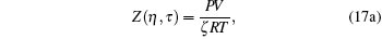
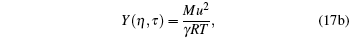
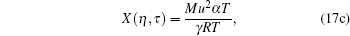
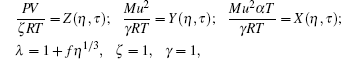
The compressibility factor Z for a fluid of Lennard– Jones molecules[15– 17] can be represented as Z(η , τ )), which contains the physical condition in terms of relation λ = g(η , f)
 |

where
 |
For graphical recreations, the above set of equations becomes
 |
 |
 |
We first assume a liquid state γ = 1 at 273.16 K, and evaluate the model parameters η and τ from the following combined equations:
 |
 |
In this way, we can easily obtain the following model parameters:
 |
 |
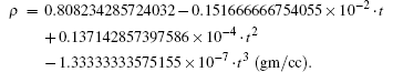
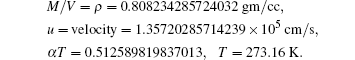
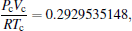
Substituting these model parameters in the basic equations of state, we can easily evaluate thermodynamic scalar variable ζ ,
 |
However, the deviation parameter ζ does not come out to unity as we expect. Hence, we should declare that the equation is mathematically exact, but physically fails to accommodate the thermodynamic data profile. We check the basic formulation or domain of such equations of state and relax or modify any physical property relating conditions so that the equations of state have some additional parameter, which explains or throws some light on the problem, then we could say some aspects are more within logical extensions. With the help of λ , we can explore the situation by evaluating the internal parameter or variable such as f. It is observed that when we select f suitably, we can use the equations to reproduce the computer simulation result in the neighborhood of the critical temperature. Note that f = 0 represents an original boundary condition.
4. Numerical results
4.1. Numerical computation and few aspects of real fluid
We assume the following functional form of λ :
 |
which is already tested in the light of the computer simulation result for the equation of state for Lennard– Jones fluids. If we assume other forms of function, such as
 |
then our maple code returns no solution, even if we run the program for 75000 s. If we search the solution under constraints such as η 1, there is no solution. The form
 |
does yield a solution, but it has poor computer simulation reproducibility in the vicinity of the critical temperature. With standard values ζ = 1, γ ≈ 1 and solving a set of equations for η , f, and τ
 |
 |
 |
we have the following form of solution:

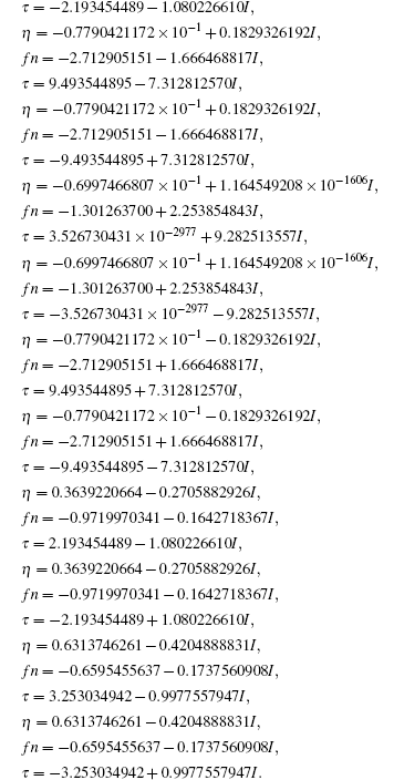
4.2. Numerical solution at 273.16 K for real fluid
It is better to represent the numerical representation of the solution in Maple format than a conventional table format
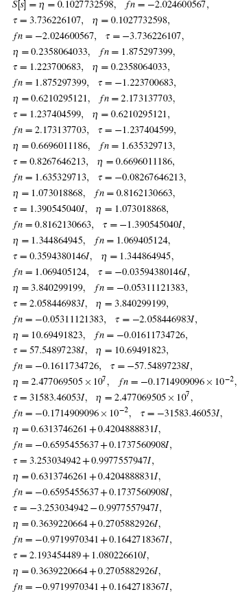
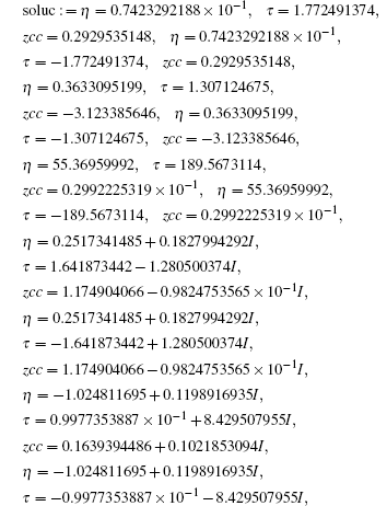
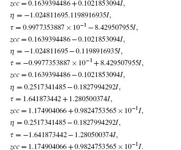
We select a few real solutions by rejecting complex solutions in the first instant for simple physical interpretation, see Table 1. The corresponding critical constants are
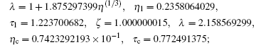
and the reduced parameters are

due to the input
| Table 1. State of a fluid corresponding to real solution S[s]. |
4.3. Graphical representation of solution at 273.16 K for real fluid
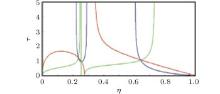
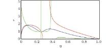
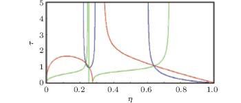
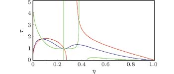
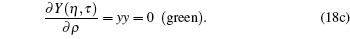
For visualization, we show Z(η , τ ) by red, Y(η , τ ) by blue, and X(η , τ ) by green. Looking at the intersections, we feels that they might represent two eigen states, as shown in Fig. 1.
4.4. Numerical representation of solution at critical temperature for real fluid
The equation of state with the first set of critical constants (η = 0.07423292188, τ = 1.772491374) is
which is closer to the experimental expectation. This is justified by the intersection of red, blue, and green curves. Another set of critical constants η =0.3633095199, τ =1.307124675 leads to

The second set of critical constants should be rejected, as supported by the following plot. Observing the intersection of (blue, green) and (green, red) curves and using a graphical language, we have
 |
 |
 |
4.5. Numerical representation of solution at critical temperature for real fluid
We have many solutions for critical contants corresponding to f = 1.875297399 in the following form:

Hence we have the following set of critical constants corresponding to f = 1.875297399. Once again it is better to represent the numerical representation of the solution in Maple format than a conventional table format
4.6. Generalization
We have the following general set of equations containing thermodynamic reduced variables [η , τ , f]:
where v is the volume of cavity containing chemical units, V is the molar volume, P is the standard pressure, ρ = N/V is the number density, T is the temperature, ε is the binding energy of the cluster containing chemical units, f is to be determined, and KB is the Boltzmann constant.
5. Conclusion
For the gas phase, we have ζ = 1, γ ≥ 1 and η → 0, τ → ∞ , while in a liquid state, the molecule can select one of the possible solutions as there is more than one solution for new parameter f and the corresponding critical constants can be calculated using Maple18. Note that the conclusion is too short and too simple because the computations are at a fixed temperature and not over the entire liquid state. On computations at different temperatures, [17] the size of the cavity rapidly decreases as the temperature of liquid increases. In the case of water, it is observed that the size of the cavity rapidly decreases as the temperature of the liquid increases.
Reference
| 1 |
|
| 2 |
|
| 3 |
|
| 4 |
|
| 5 |
|
| 6 |
|
| 7 |
|
| 8 |
|
| 9 |
|
| 10 |
|
| 11 |
|
| 12 |
|
| 13 |
|
| 14 |
|
| 15 |
|
| 16 |
|
| 17 |
|
| 18 |
|
| 19 |
|