Reception pattern influence on magnetoacoustic tomography with magnetic induction*
Cite this Article
Sun Xiao-Dong, Wang Xin, Zhou Yu-Qi, Ma Qing-Yu, Zhang Dong. Reception pattern influence on magnetoacoustic tomography with magnetic induction* . Chinese Physics B, 2015, 24(1): 014302 
Permissions
Reception pattern influence on magnetoacoustic tomography with magnetic induction*
Corresponding author. E-mail: maqingyu@njnu.edu.cn
Project supported by the National Basic Research Program of China (Grant No. 2011CB707900), the National Natural Science Foundation of China (Grant Nos 11274176 and 11474166), and the Priority Academic Program Development of Jiangsu Higher Education Institutions, China.
Abstract
Based on the acoustic radiation theory of a dipole source, the influence of the transducer reception pattern is studied for magnetoacoustic tomography with magnetic induction (MAT-MI). Numerical studies are conducted to simulate acoustic pressures, waveforms, and reconstructed images with unidirectional, omnidirectional, and strong directional transducers. With the analyses of equivalent and projection sources, the influences of the model dimension and the layer effect are qualitatively analyzed to evaluate the performance of MAT-MI. Three-dimensional simulation studies show that the strong directional transducer with a large radius can reduce the influences of equivalent sources, projection sources, and the layer effect effectively, resulting in enhanced pressure and improved image contrast, which is beneficial for boundary pressure extraction in conductivity reconstruction. The reconstructed conductivity contrast images present the conductivity boundaries as stripes with different contrasts and polarities, representing the values and directions of the conductivity changes of the scanned layer. The favorable results provide solid evidence for transducer selection and suggest potential practical applications of MAT-MI in biomedical imaging.
Keyword:
43.80.Ev; 72.55.+s; 73.50.Rb; magnetoacoustic tomography with magnetic induction (MAT-MI); reception pattern; projection source and equivalent source; layer effects
1. Introduction
As a noninvasive electrical impedance imaging modality based on coupling of multi-physics fields, magnetoacoustic tomography with magnetic induction (MAT-MI)[1, 2] uses the acoustic signals collected by the transducer around the object to reconstruct the conductivity distribution of the scanned layer. Combining the good contrast of electrical impedance tomography (EIT) and the high spatial resolution of ultrasonography, MAT-MI has great prospects in the biomedical imaging area.[3– 5] Since MAT-MI was first proposed by Yuan Xu and Bin He in 2005, many relevant works have been carried out all around the world. Hu et al.[6] reported an experimental study on magnetoacoustic imaging of superparamagnetic iron oxide (SPIO) nanoparticles embedded in biological tissues, providing a promising tool for the tomographic reconstruction of magnetic nanoparticle-labeled diseased tissues in molecular or clinical imaging. Mariappan et al.[7] proposed a conductivity reconstruction method based on vector acoustic source imaging and obtained a reliable conductivity estimation with the proposed reconstruction method. Different from the previous researches using isotropic conductive models, Li et al.[8] studied the forward problem of MAT-MI for the conductivity anisotropy model with the aid of the finite element method (FEM). Mariappan et al.[9] demonstrated that imaging resolution and contrast for the biological tissue conductivity reconstruction of MAT-MI can be well improved under an MRI using a high static magnetic field environment.
Owing to the same source distribution of each layer, cylindrical phantom models were chosen to simplify experiments and simulations.[10– 13] The experimental images of MAT-MI for the cylindrical models were provided and the reconstructed conductivity contrast images agreed well with the real conductivity distributions of the scanned layers.[5, 14] As the experimentally used transducer had a strong directivity due to its large surface radius, two-dimensional (2D) and three-dimensional (3D) simulation results usually coincided well with the experimental results. However, additional wave clusters and image artifacts were still observed clearly without a reasonable explanation and less attention has been focused on the pivotal role of the transducer reception pattern in the 2D measurement configuration of MAT-MI.
In MAT-MI, a transducer with an ideal reception pattern[15] can only detect acoustic signals transmitted along the normal direction of the transducer surface. The information of the acoustic source strength, vibration polarity, and the location of conductivity boundaries can be easily extracted from the collected signals, which is beneficial for the conductivity reconstruction of the scanned layer. Considering the 3D acoustic transmission of the dipole source and the reception pattern of the transducer, the detected pressure should be calculated as the superposition of all the transmitted signals from the sources inside the object in a limited reception angle scope. Therefore, besides the sources of the scanned layer, the influence of the layer effects[16] cannot be ignored, resulting in image artifacts with reduced accuracy of pressure identification and source localization. However, even though several investigations of how to compensate for transducer directivity in photoacoustic tomography have been reported, [17, 18] no special studies about the production, influence, and solution of MAT-MI have been published in the previous studies.
In this paper, based on the theory of acoustic dipole radiation, the influence of the transducer reception pattern on MAT-MI is investigated with 3D numerical simulations of acoustic pressure, waveform, and image reconstruction using unidirectional, omnidirectional, and strong directional transducers. Based on the analyses of the equivalent source and the projection source, the generations of abrupt and gentle pressure changes and additional pressure variations are qualitatively discussed. With various reception patterns, the influences of model dimensions and layer effects on detected pressures and reconstructed images are also analyzed. The favorable results provide the bases for transducer selection and suggest the feasibility of boundary pressure extraction for the conductivity image reconstruction with MAT-MI.
2. Principles and methods
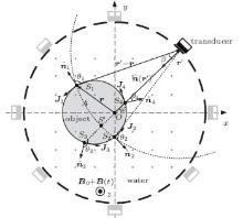
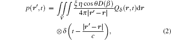
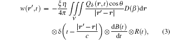
The schematic diagram of MAT-MI is illustrated in Fig. 1. An object with conductivity distribution σ (r) is placed in a complex magnetic field composed of a static magnetic field B0 = B0ẑ and a time-varying magnetic field B(t) = B(t)ẑ . For simplicity, the magnetic field is assumed to be homogeneous, covering the whole object. Induced by B(t), eddy currents J(r, t) appear in close loops on each layer parallel to the xy plane inside the object. With the interaction between B0 and J(r, t), the medium at r is exerted by Lorentz force J(r, t)× B0 to produce an acoustic vibration. Centered at the origin, the transducer travels around the object to detect acoustic signals transmitted from all vibration sources inside the object, which can be used to reconstruct the conductivity distribution for the scanned layer. Therefore, at the observation point r′ around the object, the acoustic pressure satisfies the wave equation[1– 5, 19]
 |
where p(r′ , t) is the acoustic pressure at observing point r′ , ∇ 2 and ∇ are the Laplacian and the divergence operator, respectively, and c is the acoustic speed in the media.
 | Fig. 1. Schematic diagram of MAT-MI. |
To simplify the principle derivation, the pulsed magnetic field is set to be a step function as B(t) = ε (t)ẑ , then the induced electric field Eδ (r, t) satisfies ∇ × Eδ (r, t) = − δ (t)ẑ and the acoustic source strength can be expressed as Qδ (r, t) = ∇ ˙ [Jδ (r, t)× B0]. Therefore, the acoustic pressure detected at the observation position r′ can be described as[13, 20– 22]
 |
where ⊗ is the convolution operator, r and r′ are the positions of the acoustic source and the receiver, respectively, ξ is the pressure conversion efficiency of the transducer, η = − jkΔ r = − j2π Δ r/λ is a dimensionless constant[13] determined by the fixed wavelength λ and the distance Δ r between the two monopole sources of each acoustic dipole, and θ is the radiation angle between the transmission path (r′ − r) and the normal direction 

The acoustic waveform w(r′ , t) collected at r′ can be obtained as the convolution result[11] between p(r′ , t) and the system transfer function h(t) = − [dB(t)/dt]⊗ R(t) as
 |
where R(t) and B(t) are the waveforms of the transducer impulse response and the pulsed magnetic field, respectively. Based on the simplified back projection algorithm[22] for diffraction sources, the 2D cross sectional conductivity contrast image of the scanned layer can be reconstructed with the waveforms collected around the object
 |
where I(r) is the reconstructed intensity at source position r and φ is the measure angle of the transducer.
3. Numerical simulations
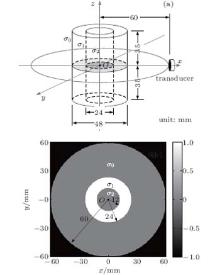
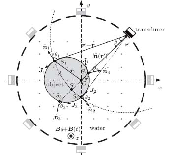
To verify the influence of the reception pattern on MAT-MI, numerical simulations were conducted with a two-layer coaxial cylindrical model. Figures 2(a) and 2(b) illustrate the 3D diagram of the model and the cross sectional conductivity distribution for z=0, respectively. The height of the model was set to be 70 mm, and the radii of the outer and the inner media were set to be 24 mm and 12 mm, respectively. The conductivities of the outer and the inner media were σ 1 = 1 S/m and σ 2 = 0 S/m. Both the transducer and the model were placed in distilled water with conductivity σ 0 = 0 S/m for acoustic coupling. The transducer moved around the model in a circular orbit centered at the origin with a radius of 60 mm to collect acoustic waveforms. For simplicity, the acoustic impedances of the media were assumed to be homogeneous to ignore acoustic reflection, dispersion, and attenuation. The acoustic velocity and the calculation grid were set to be 1500 m/s and 0.3 mm at the sampling rate of 5 MHz. In order to improve the comparability between numerical simulations and experimental results, the actual waveforms of the impulse response of the transducer R(t) and the differential of the pulsed magnetic field dB(t)/dt were used in the simulation studies. The system transfer function h(t) of the MAT-MI experimental system was a three-cycle damping wave cluster at the center frequency of 0.5 MHz.[19]
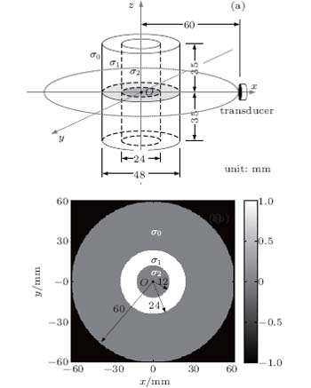 | Fig. 2. Illustration of the two-layer coaxial cylindrical model: (a) 3D diagram of the model, (b) the cross sectional conductivity distribution for z = 0. |
3.1. Equivalent source analysis
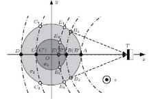
The cross sectional diagram of the two-layer cylindrical model is shown in Fig. 3. For the transmission time t, the detected pressure is the summation for all the sources on the source arc with the transmission distance ct, whcih can be considered as one equivalent source on the normal direction of the transducer. For example, the sources on arc B1BB2 can be equivalent to source B′ with the time delay of | BT| /c, while the source arc E1E2EE3E4 can be equivalent to source E′ with a longer time delay of | ET| /c.
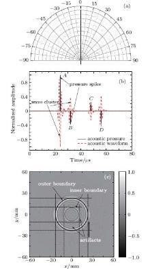
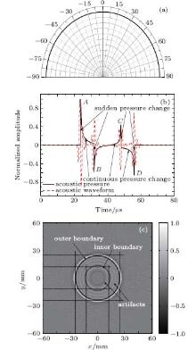
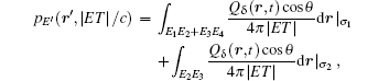
For acoustic detection, the pressure is closely related with the reception pattern of the transducer. Figure 4(a) describes the ideal reception pattern of a unidirectional transducer, [15] indicating that only the pressure transmitted along the normal direction of the transducer can be detected. So for the 2D measurement configuration in Fig. 3, only four pressure spikes at 24 μ s, 32 μ s, 48 μ s, and 56 μ s are obtained as shown in Fig. 5(b) (solid line), corresponding to the four sources A, B, C, and D located at the conductivity boundaries along the normal direction of the transducer. For the sources with the radiation angles 0 and π , the pressure amplitudes are determined by the source strengths, the transmission distances, and cosθ . Positive and negative pressure polarities imply the conductivity changes of 1→ 0 S/m and 0→ 1 S/m at the conductivity boundaries. By convoluting the detected pressure with the system transfer function, the collected waveform is obtained as presented in Fig. 4(b). The time delays, amplitudes, and phases of the wave clusters agree well with the corresponding pressure spikes, reflecting the information of conductivity changes at the boundaries.
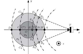 | Fig. 3. Analysis diagram of 2D equivalent sources for the cross section of the two-layer cylindrical model. |
With the simulated waveforms collected around the model, a 2D conductivity contrast image was reconstructed as shown in Fig. 4(c). Two obvious circles in stripes with different radii, contrasts, and polarities represent the inner and the outer conductivity boundaries of the scanned layer, which agree well with the configuration in Fig. 2(b) in terms of shape and size. Suppose that the polarity of the outer circular borderline stripe is positive, corresponding to the conductivity change of 0 → 1 S/m, then it is negative for the inner stripe with the conductivity change of 1 → 0 S/m. Therefore, opposite directions of conductivity changes at the media boundaries can be identified from the reconstructed conductivity contrast image. However, besides the two conductivity boundary circles, several artifacts introduced by the system transfer function are visualized, resulting in reduced spatial resolution and image quality.
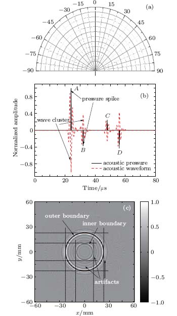 | Fig. 4. 2D simulations with a unidirectional transducer: (a) reception pattern, (b) pressure and waveform, (c) reconstructed conductivity contrast image. |
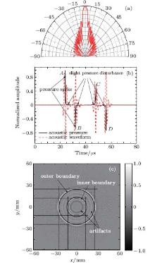
In practical applications, the reception pattern of the commonly used planar piston transducer is mainly determined by the frequency and the radius. For a transducer with an infinitesimal radius of ka ≪ 1, D(β ) ≡ 1 and the corresponding hemispherical omnidirectional reception pattern in Fig. 5(a) indicates that the transducer can detect the acoustic pressures transmitted in the reception angle from − π /2 to π /2 without any direction attenuation. As displayed in Fig. 3, the source A at the outer boundary has the shortest transmission distance | AT| and produces the first positive pressure at time | AT| /c. While the source D has the same source strength and an opposite vibration direction, producing the last negative pressure with the longest time delay | DT| /c. For the source arc B1BB2, sources from B1 to B2 in the outer medium have the same distance | BT| and the pressure of the equivalent source B′ can be calculated by

This is also the case for the source arc C1CC2. In addition, for the source arc E1E2EE3E4 with the transmission distance | ET| , the equivalent source E′ can be considered as the summation of all the sources in the outer and the inner media as
where the first and the second terms are calculated for the two conductive homogeneous media with the conductivities σ 1 and σ 2, respectively.
 | Fig. 5. 2D simulations with an omnidirectional transducer: (a) reception pattern, (b) pressure and waveform, (c) reconstructed conductivity contrast image. |
The simulated pressure of the two-layer cylindrical model detected using an omnidirectional transducer is depicted in Fig. 5(b). Compared with Fig. 4(b), four abrupt pressure changes at 24 μ s, 32 μ s, 48 μ s, and 56 μ s are observed, reflecting the positions and the polarities of the conductivity changes at A, B, C, and D. Meanwhile, owing to the omnidirectional reception pattern, the amplitudes of the pressure spikes B, C, and D are enhanced and gentle pressure changes appear between adjacent spikes, which can be explained by the continuously distributed equivalent sources with different transmission distances. Despite the obvious differences between the pressures, similar waveforms are obtained in Figs. 4(b) and 5(b). Four wave clusters are consistant with the abrupt pressure changes in amplitude and phase. Due to the convolution effects, no cluster can be observed corresponding to the gentle pressure changes. Similar to Fig. 4(c), the reconstructed image in Fig. 5(c) shows the cross sectional conductivity boundaries of the model with opposite borderline stripes. Furthermore, an improved image contrast with reduced artifacts is identified.
 | Fig. 6. 2D simulations with a strong directional transducer: (a) reception pattern, (b) pressure and waveform, (c) reconstructed conductivity contrast image. |
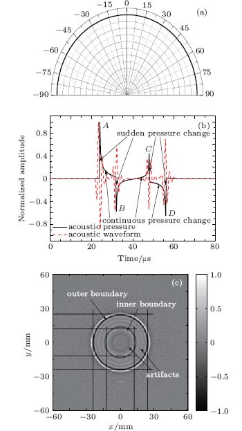
For the experimental transducer (center frequency 0.5 MHz, diameter 38 mm), a strong directional reception pattern with a main lobe of about ± 8° is achieved as shown in Fig. 6(a). The simulated pressure displayed in Fig. 6(b) is similar to that in Fig. 4(b). Corresponding to the conductivity boundaries A, B, C, and D, four pressure spikes are clearly displayed. Owing to the narrow angle scope of the main lobe, gentle pressure changes between adjacent spikes are greatly attenuated. Meanwhile, slight pressure disturbances near each spike can also be identified, which are produced by the side lobes of the reception pattern. In addition, the relative amplitudes of the pressure spikes B, C, and D are enhanced due to the wider source arcs of longer transmission distances. Therefore, four wave clusters with opposite phases and enhanced amplitudes are achieved in Fig. 6(b), and the small clusters induced by the slight pressure disturbances can hardly be distinguished from the adjacent boundary clusters. The reconstructed image displayed in Fig. 6(c) shows good consistency with those in Figs. 4(c) and 5(c) in the shape, size, and polarity of the borderline stripes. The image contrast of the boundary borderline stripes is improved obviously with reduced artifacts.
3.2. Projection source analysis
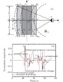
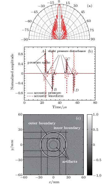
In MAT-MI, each Lorentz force induced acoustic dipole source generates a 3D acoustic radiation, and the detected pressure is the summation for the sources in all layers of the model. The acoustic sources on the layers at different heights can be equivalent to projection sources on the scanned layer, and the projection sources can be further simplified to equivalent sources along the normal direction of the transducer. The diagram of the projection sources for the longitudinal section of the two-layer cylindrical model is shown in Fig. 7(a). The transducer is placed on the middle layer at z=0 to detect the acoustic signal transmitted from the longitudinal section. The detected pressure produced by the sources in each layer is determined by the height, which has a great impact on the transmission distance and the radiation angle. Considering the different transmission distances, the boundary sources A1, B1, C1 , and D1 at z = − h can be regarded as the projection sources A′ , B′ , C′ , and D′ . The distances from the transducer to the projection sources are longer than those to the corresponding boundary sources of the scanned layer. For example, | A′ T| is longer than | AT| and it introduces an additional time delay (| A′ T| − | AT| )/c. By taking the superposition for all the layers, the pressure detected with an omnidirectional transducer is shown in Fig. 7(b). Four abrupt pressure changes at 24 μ s, 32 μ s, 48 μ s and 56 μ s are displayed, representing the conductivity boundaries A, B, C, and D of the scanned layer, respectively. Gentle pressure changes with positive and negative polarities appear due to the continuous distribution of the dipole sources. Meanwhile, several additional pressure variations AH, BH, CH, and DH with the time delays of 33.2 μ s, 39.3 μ s, 53.1 μ s, and 60.4 μ s are visualized, corresponding to the boundaries AH1, BH1, CH1, DH1 for z = H and AH2, BH2, CH2, DH2 for z = − H. Therefore, besides four wave clusters A, B, C, and D, four additional clusters with relatively lower amplitudes are found in the waveform. The clusters BH, CH, and DH at 39.3 μ s, 53.1 μ s, and 60. 4 μ s are visualized distinctly, while the cluster AH can hardly be distinguished from the adjacent cluster B. Due to the existence of the additional clusters, the spatial resolution of the reconstructed image is reduced with more artifacts.
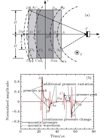 | Fig. 7. (a) Diagram of projection sources, (b) pressure and waveform for the longitudinal section of the two-layer coaxial cylindrical model with an omnidirectional transducer. |
3.3. Layer effects analysis
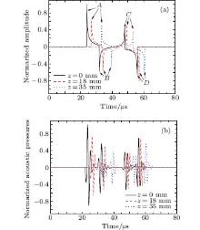
To investigate the layer effects of MAT-MI, the detected pressures produced by the acoustic sources on the layers at z=0 mm, 18 mm, and 35 mm are simulated using an omnidirectional transducer as shown in Fig. 8(a). Four pressure spikes denoting the four boundaries on each calculation layer are displayed. For z = 0 mm, the times of the pressure peaks A and D at 24 μ s and 56 μ s represent the transmission distances of 36 mm and 84 mm for the corresponding sources, and the distance of 48 mm reflects the diameter of the outer medium. So are the cases for the pressure peaks B and C with the time delay of 16 μ s, corresponding to the diameter of 24 mm of the inner medium. With the increase of z, extended time delays and strengthened pressure attenuations of the pressure peaks are also observed. For z= 18 mm, the times of the pressure peaks A and D are 26.8 μ s and 57.3 μ s, reflecting the distance of 45.6 mm, which is smaller than the actual diameter of the outer medium. For z = 35 mm, the times of the pressure peaks A and D increase to 33.5 μ s and 60.7 μ s with a decreased distance of 40.8 mm. The corresponding waveforms for the layers of z=0 mm, 18 mm, and 35 mm are shown in Fig. 8(b). Four wave clusters are clearly displayed, denoting the four boundaries of the calculated layers with corresponding time delays and amplitudes.
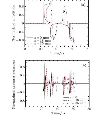 | Fig. 8. 2D simulations with an omnidirectional transducer for the layers at z=0 mm, 18 mm, and 35 mm: (a) pressure, (b) waveforms. |
3.4. 3D simulation studies
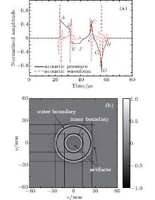
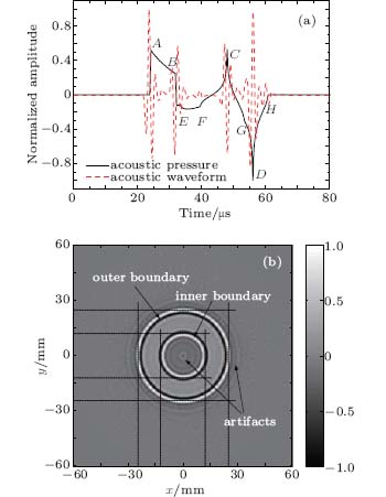
By combining the analyses of equivalent source, projection source, and layer effects, 3D numerical studies for the two-layer cylindrical model were conducted and the simulated results using an omnidirectional transducer are shown in Fig. 9(a). Influenced by the dimension and layer effects of the model, the detected pressure is quite different from those in Figs. 5(a), 6(b), and 8(a) in shape and amplitude. However, four abrupt pressure changes A, B, C, and D at 24 μ s, 32 μ s, 48 μ s, and 56 μ s still present the exact locations of the four conductivity boundaries of the scanned layer. Produced by the projection sources and the layer effects, abrupt pressure changes E, F, G, and H at about 33 μ s, 44 μ s, 53 μ s, and 60 μ s are also identified. From the simulated waveform in Fig. 9(a), four wave clusters with opposite vibration phases are clearly observed, corresponding to the abrupt pressure changes of A, B, C, and D. Meanwhile, two small clusters generated by the abrupt pressure changes F and H are also visualized. Overlapped with the clusters B and D, the clusters produced by the abrupt pressure changes E and G can hardly be differentiated. In Fig. 9(b), the reconstructed image agrees well with the conductivity configuration in Fig. 2(b). The conductivity boundaries of the outer and the inner media are displayed as positive and negative borderline stripes with improved contrast, representing the opposite conductivity changes of 1 → 0 S/m and 0 → 1 S/m. Owing to the existence of the clusters F and H, two additional stripes near the origin and outside the outer borderline are also visualized as image artifacts.
 | Fig. 9. 3D simulations with an omnidirectional transducer for the two-layer cylindrical model: (a) pressure and waveform, (b) reconstructed conductivity contrast image. |
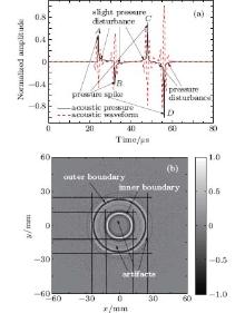
Figure 10(a) illustrates the 3D simulated pressure and waveform using a strong directional transducer for the two-layer cylindrical model. Due to the strong directivity of the transducer, the pressure distribution is similar to that detected by a unidirectional transducer in Fig. 4(b). Owing to the side lobes of the reception pattern, slight pressure disturbances are observed, which are close to the pressure spikes of the boundaries A, B, C, and D of the scanned layer. What is more, with the increase of the time delay, the relative pressure amplitudes of the spikes are enhanced obviously. Therefore, only four wave clusters with opposite vibration phases are in existence, and the tiny clusters produced by the slight pressure disturbances are too weak to be identified. An improved image contrast with reduced artifacts can be obtained from the reconstructed conductivity contrast image as shown in Fig. 10(b).
 | Fig. 10. 3D simulations with a strong directional transducer for the two-layer cylindrical model: (a) pressure and waveform, (b) reconstructed conductivity contrast image. |
4. Discussion
Assuming that the transducer has an omnidirectional reception pattern, the distributions of the detected pressures are affected greatly by the model dimensions, especially by the model height. (i) For a short model, the projection sources of the top and the bottom layers are close to the corresponding sources of the scanned layer, producing superimposed pressures and clusters. The 3D simulation is approximate to the 2D one, and the reconstructed image can be regarded as the conductivity contrast image of the scanned layer. (ii) With the increase of the model height, the detected pressures generated by the sources of the top and the bottom layers are separated from those generated by the scanned layer, which will introduce additional wave clusters and result in boundary artifacts and reduced spatial resolution for the image reconstruction. (iii) If the model height is increased to an infinite value, the detected pressures generated by the sources of the top and the bottom layers tend to be zero due to the radiation angle of π /2. Therefore, only the wave clusters corresponding to the conductivity boundaries of the scanned layer can be achieved and no additional boundary artifacts will be produced.
The detected pressure is also influenced greatly by the reception pattern of the transducer. (i) For an ideal unidirectional reception pattern, only the acoustic signals transmitted along the normal direction of the transducer can be detected. The conductivity contrast image of the scanned layer can be reconstructed and the influence of the model dimensions can be neglected. (ii) For an omnidirectional reception pattern, acoustic signals produced by sources on all layers within the entire object can be detected without directional attenuation. Besides the abrupt pressure changes generated by the boundary sources, gentle pressure changes produced by equivalent and projection sources can also be detected. Additional pressure disturbances introduced by the model dimensions and the layer effects can be detected, resulting in additional boundary artifacts and a reduced spatial resolution for the image reconstruction. (iii) For a strong directional reception pattern, only the signals transmitted in a limited angle scope can be detected with corresponding pressure attenuation. Pressure peaks appear in the form of sharp spikes, approaching the results of the ideal reception pattern. Therefore, the strong directional reception pattern can effectively reduce the influences of equivalent sources, projection sources, and layer effects, leading to an enhanced pressure contrast and reduced image artifacts.
In most previous studies[1– 4, 6, 7, 9, 11, 13, 15, 16] of MAT-MI experiments, planar piston transducers with a radius of about 1– 3 cm were used as the receiver to detect the acoustic pressure. Although the conductivity boundary of the scanned layer can be presented in the reconstructed images, the broad borderline stripes are observed with reduced image resolution and contrast, and the conductivity changes cannot be reflected accurately by the amplitudes of the boundary stripes due to the influence of the transducer reception pattern. In addition, the artifacts introduced by the side lobe of the transducer can also be seen in the reconstructed images with reduced image quality. The problems can be explained well with the proposed theories of equivalent and projection sources in this paper. To enhance the directivity of the transducer, Xia et al.[5] and Li et al.[12] conducted their MAT-MI experiments with focused transducers and the spatial resolutions of the reconstructed images were enhanced, which are beneficial for the quantitative conductivity reconstruction in MAT-MI. In addition, considering the high spatial resolution and the improved contrast of the ultrasound imaging with a sector array transducer, [24] the application of the sector array transducer might be employed in further studies of MAT-MI.
5. Conclusion
Based on the acoustic dipole radiation theory, the influences of the transducer reception pattern on MAT-MI are studied with a two-layer cylindrical phantom model in this paper. Numerical studies for acoustic pressures, waveforms, and reconstructed images using unidirectional, omnidirectional, and strong directional transducers are performed with the analyses of equivalent source, projection source, and layer effects. The generations of abrupt and gentle pressure changes, additional pressure disturbances, as well as the influences on the image reconstruction are discussed qualitatively. The reconstructed conductivity contrast image indicates the conductivity boundaries of the scanned layer as stripes with different contrasts and polarities, representing the values and directions of the conductivity changes. A strong directional transducer can effectively reduce the influence of equivalent source, projection source, and layer effects, resulting in the enhanced pressures, an improved image contrast, and reduced artifacts, which are beneficial for boundary pressure extraction in conductivity reconstruction. The favorable results provide numerical evidence for transducer selection and suggest potential practical applications of MAT-MI in biomedical imaging.
The authors would like to thank Prof. Bin He (Department of Biomedical Engineering, University of Minnsota, USA) for his guidance in the research on MAT-MI and thank Prof. Juan Tu (Institute of Acoustics, Nanjing University, China) for her assistant in paper preparation.
Reference
| 1 |
|
| 2 |
|
| 3 |
|
| 4 |
|
| 5 |
|
| 6 |
|
| 7 |
|
| 8 |
|
| 9 |
|
| 10 |
|
| 11 |
|
| 12 |
|
| 13 |
|
| 14 |
|
| 15 |
|
| 16 |
|
| 17 |
|
| 18 |
|
| 19 |
|
| 20 |
|
| 21 |
|
| 22 |
|
| 23 |
|
| 24 |
|