Hybrid natural element method for viscoelasticity problems<xref ref-type="fn" rid="cpb142038fn1">*</xref>

Cite this Article

Zhou Yan-Kai, Ma Yong-Qi, Dong Yi, Feng Wei. Hybrid natural element method for viscoelasticity problems* . Chinese Physics B, 2014, 24(1): 010204 Copy to clipboard

Permissions

Hybrid natural element method for viscoelasticity problems*

Zhou Yan-Kai^a), Ma Yong-Qi^a),^b)†, Dong Yi^c), Feng Wei^a)

a)Shanghai Institute of Applied Mathematics and Mechanics, Shanghai University, Shanghai 200072, China

b)Department of Mechanics, Shanghai University, Shanghai 200444, China

c)Shanghai Industrial Urban Development Group Limited, Shanghai 200030, China

†Corresponding author. E-mail: mayq@staff.shu.edu.cn

*Project supported by the Natural Science Foundation of Shanghai, China (Grant No.13ZR1415900).

Abstract

A hybrid natural element method (HNEM) for two-dimensional viscoelasticity problems under the creep condition is proposed. The natural neighbor interpolation is used as the test function, and the discrete equation system of the HNEM for viscoelasticity problems is obtained using the Hellinger–Reissner variational principle. In contrast to the natural element method (NEM), the HNEM can directly obtain the nodal stresses, which have higher precisions than those obtained using the moving least-square (MLS) approximation. Some numerical examples are given to demonstrate the validity and superiority of this HNEM.

Keyword: 02.60.Cb; 02.60.Lj; 46.35.+z; hybrid natural element method; viscoelasticity; Hellinger–Reissner variational principle; meshless method

Show Figures

1. Introduction

The meshless method is a numerical method that is an alternative to the finite element method (FEM). The trial function of the meshless method is constructed from a set of nodes, which allows the meshless method not to generate a mesh, so it will save more preliminary workload than the FEM. It has been given great attention by many researchers since the element-free Galerkin (EFG) method was presented by Belytschko.^[1] In addition to the EFG method, ^{[2, 3]} there are many other meshless methods, such as the improved element-free Galerkin method, ^{[4– 7]} the complex variable meshless method, ^{[8– 10]} the complex variable element-free Galerkin (CVEFG) method, ^{[11– 17]} the interpolating element-free Galerkin (IEFG) method, ^{[18, 19]} the radial basis function (RBF) method, ^[20] the finite point method (FPM), ^{[21, 22]} the meshless local Petrov– Galerkin (MLPG) method, ^[23] the reproducing kernel particle method (RKPM), ^{[24– 28]} the meshless manifold method, ^{[29, 30]} the boundary element-free method (BEFM), ^{[31– 40]} and the improved boundary element-free method (IBEFM).^{[41– 44]}

The natural element method (NEM) is a meshless method, first presented by Braun and Sambridge; ^[45] this method has been successfully applied in solid mechanics and fluid mechanics. Sukumar et al.^[46] successfully solved partial differential equations of the elliptic type in solid mechanics by using this method. Bueche et al.^[47] researched the NEM for elastokinetics problems. Cueto et al.^[48] extended the NEM based on the concept of an a -shape and realized a three-dimensional analysis. Matinez et al.^[49] applied the NEM in the analysis of fluids. Calvo et al.^[50] studied the NEM for large deformation problems. Daneshmand and Niroomandi discussed the vibration modes of fluid-structure systems using the NEM.^[51] Daneshmand et al.^[52] used the NEM to calculate the two-dimensional flow under sluice gates. Shahrokhabadi et al.^[53] used the NEM to analyze seepage problems of underground water. The natural element approximation of the Reissner– Mindlin plate for locking-free numerical analysis of plate-like thin elastic structures was established by Cho et al.^[54]

Because the test functions of the NEM are smooth (C^∞ )except at the nodes where they are C⁰, ^{[55– 57]} we cannot obtain the nodal stresses. To overcome this disadvantage, we can use the MLS approximation to calculate the nodal stresses by the nodal displacements obtained using the NEM. This method was first used in the FEM by Tabbara et al.^[58] Except for this method, the hybrid natural element method (HNEM) can also obtain the nodal stresses, which has been successfully applied in elasticity problems and elastoplasticity problems.^{[59, 60]} The HNEM adopts displacement interpolation and stress interpolation respectively using natural neighbor interpolation, ^{[61, 62]} and the corresponding formulae are obtained according to the Hellinger– Reissner variational principle.^{[63, 64]}

Viscoelasticity problems are important nonlinearity problems in material engineering. Viscoelastic materials have the characteristics of both an elastic solid and a viscous fluid, so the stress– strain relationship is difficult to model. Peng and Xu studied the constitutive relationship of permanent deformation in asphalt pavements.^[65] The constitutive relationship of viscoelastic materials correlates with time. Thus the effect of time on the material should be considered in the calculation. That the time parameter is important in the process of calculation brings great difficulty in solving the viscoelasticity mechanics problems, so analytical solutions can be obtained for only a few simple viscoelastic problems.^[66] The solutions of complex viscoelastic problems in engineering mainly rely on numerical calculations, for which the meshless methods have been widely used. Yang and Liu combined the element-free Galerkin method and a precise algorithm in the time domain to study two-dimensional viscoelasticity problems.^[67] Using the meshless local Petrov– Galerkin method, Sladek et al.^{[68, 69]} analyzed anisotropic and linear viscoelastic solids, and discussed quasistatic and transient dynamic problems in two-dimensional linear viscoelastic media. Based on the rigid/viscoplastic element-free Galerkin method, the massive metal forming process was discussed by Guan et al.^[70] Canelas and Sensale studied a boundary knot method for harmonic elastic and viscoelastic problems.^[71] A complex variable element-free Galerkin method for linear viscoelasticity problems under the creep condition was analyzed by Cheng et al.^[72] Three-dimensional viscoelasticity problems were analyzed via the improved element-free Galerkin method by Peng et al.^[73]

Based on the natural neighbor interpolation, the HNEM for two-dimensional viscoelasticity problems under the creep condition is presented in this paper. According to the linear viscoelastic Hellinger– Reissner variational principle, the equation system of the viscoelastic hybrid natural element method under the creep condition is established. Finally, the effectiveness and superiority of this method are proved through numerical examples in this paper.

2. The shape functions for the HNEM

The natural neighbor interpolation (NNI)^{[61, 62]} in the NEM is adopted to construct the shape functions for the HNEM. Consider a bounded domain Ω in two dimensions that is described by a set N of m scattered nodes: N = {N₁, N₂, . . . , N_m}, m ≥ 3; their coordinates are x_i, i = 1, 2, . . . , m. The Voronoi diagram V ( N) of the set N is a subdivision of the domain into regions V ( N_i) , where each region V ( N_i) is associated with a node N_i, such that any point in V ( N_i) is closer to N_i than to any other node N_j ( j ≠ i) . The Voronoi diagram in essence partitions space into closest-point regions. The region V ( N_i) (Voronoi cell) for a node N_i is a polygon

where d( x_i, x_j) is the Euclidean distance between x_i and x_j.

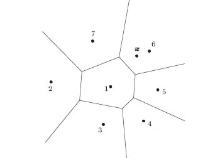
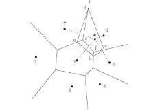
A part of the Voronoi diagram V ( N) is shown in Fig. 1. Suppose x to be any point within the region, the natural neighbor nodes around x are found according to the empty circumcircle criterion of Delaunay.^[74] The natural neighbor nodes of x are 1, 5, 6, and 7, as shown in Fig. 2.

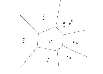	Figure Option View Download New Window
	Fig. 1. An original Voronoi diagram and x.

	Figure Option View Download New Window
	Fig. 2. The 1st-order and the 2nd-order Voronoi cells about x.

After the natural neighbor nodes of x are determined, we can build a local interpolation format as follows:

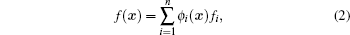where f( x) is the interpolation physical quantity for node x; i is the serial number of natural neighbor nodes around x; n is the total number of natural neighbor nodes around x; f_i is the physical quantity value of node i; and ϕ _i( x) is the shape function of node x_i. The shape function can be chosen between Sibsonian and non-Sibsonian interpolations.^[62]

The Sibsonian interpolation can be written as

where A_j( x) is the area of overlap of Voronoi cells between node j and x, and A( x) is the area of the Voronoi cell of x. The four regions shown in Fig.2 are the second-order cells, while their union (closed polygon abcd) is the first-order Voronoi cell, and the shape function ϕ ₁( x) is given by

The derivatives of ϕ _i( x) can be obtained by differentiating Eq. (3)

(6)

For the traditional mechanical problems, we can take Eq. (3) as the displacement interpolation function

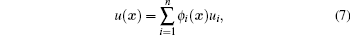where ϕ _i( x) is the shape function associated with node i, and u_i is the displacement of node i.

By definition of the shape function given in Eq. (3), we have the following relations:

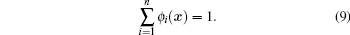Referring to Fig. 2, if x is to coincide with any node, for instance node 1, then it is readily seen that ϕ ₁( x) = 1 and ϕ _i( x) = 0, i ≠ 1, i.e.,

which implies that the natural neighbor interpolation passes through the node values, and the node unknowns u_i are the nodal displacements, which is in contrast to most meshless approximations, where the nodal parameters u_i are not the nodal displacements. Thus the essential boundary conditions can be imposed easily by using the natural neighbor interpolation, as in the FEM.

3. The HNEM for two-dimensional linear viscoelasticity problems

3.1. Constitutive relationships of linear viscoelastic materials

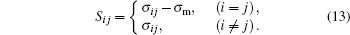
Under the condition of small deformation, the stress tensor of an isotropic material can be described as

where

The strain tensor can be similarly written as

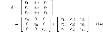where

The constitutive relationship of linear viscoelastic materials can be written as

where J₁ ( t) and J₂ ( t) are two creep compliances. The J₁ ( t) varies for different models. For the case of the Maxwell model,

for the case of the Kelvin model,

and for the case of the three-parameter model,

where G, G₁, and G₂ are the shear elastic moduli, and η is the viscosity constant of each model. The J₂ ( t) is

where K is the volumetric modulus of elasticity, and

with E being the elasticity modulus, and ν being the Poisson ratio.

3.2. The HNEM for two-dimensional viscoelasticity problems

Under the creep condition, the stress σ is constant, while the strain ε ( t) and the displacement u ( t) depend on time, as shown in Eq. (17). For the two-dimensional problems, by assuming that the body force in the problem domain Ω , the traction on the natural boundary Γ _σ, and the displacement ū of the essential boundary Γ _u are all known, the basic equations of viscoelasticity problems can be expressed as follows.

The equilibrium equation can be written as

where

The strain– displacement relationship can be written as

where

The stress– strain relationship can be written as

and the constitutive matrix C is

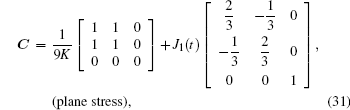where J₁ and K can be obtained from Eqs. (18)– (20) and (22).

The boundary conditions can be written as

where

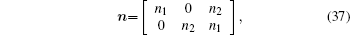and n₁ and n₂ are the units outward normal to boundary Γ _σ, respectively.

Suppose that there are N nodes in problem domain Ω , the displacement and the stress at an arbitrary point x can be expressed as

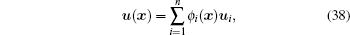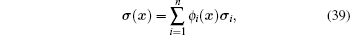where n is the total number of natural neighbor nodes around x, and ϕ _i is the interpolation function of displacement u and stress σ , which can be constructed by Eq. (3).

Equations (38) and (39) can be written in matrix form as

where Φ ( x) and P( x) are matrices of shape functions, q and β are the nodal displacement vector and the nodal stress vector, respectively,

The properties of linear viscoelastic materials are related to time only and have nothing to do with the loading history. So the stress and the displacement at each point in time can be calculated directly by the Hellinger– Reissner variational principle. At each point in time, the Hellinger– Reissner variational principle can be expressed as

where

and B is the surplus energy density function

where C can be obtained from Eqs. (31) and (32).

Supposing that the displacement boundary condition Eq. (33) is satisfied, and substituting Eqs. (40), (41), and (52) into Eq. (50), we can obtain

where

According to the stationary value condition of the multi-variation variational principle

we have

Substituting Eq. (60) into Eq. (54) yields

where

Based on the stationary condition of the variation principle, i.e.,

the equations of the HNEM for solving the generalized displacement can be found as follows:

We can obtain the nodal displacements at any time by solving Eq. (64), and the nodal stresses can be obtained by substituting the nodal displacements in Eq. (60). Then the displacement and the stress at any point in the domain can be gained using Eqs. (40) and (41). Thus the HNEM for two-dimensional viscoelasticity problems under the creep condition is established.

4. Numerical examples

Four examples are discussed to demonstrate the applicability of the HNEM for two-dimensional linear viscoelasticity problems. The results obtained using the HNEM are compared with the analytical solutions and the ones of the NEM and the FEM. The nodal stresses obtained from the NEM are calculated with the MLS approximation.

The Sibson interpolation is used as the shape function in the numerical examples presented in this section. Delaunay triangles are used as the integration cells, and in each integration cell, three Gauss points are used for the Gaussian quadrature.

4.1. Cylinder under a distributed inner pressure

A cylinder with uniform pressure p on the inner surface is shown in Fig.3, the outer radius of the cylinder is b = 5 m, and the inner radius is a = 1 m. The inner pressure is p = 30 kPa and the volume deformation is elastic, elasticity modulus E = 1.0 × 10⁶ Pa, Poisson ratio ν = 0.25. For the rheological properties of shear deformation, we respectively adopt the Maxwell model and the Kelvin model, and the parameters are

	Figure Option View Download New Window
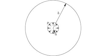	Fig. 3. Cylinder under a distributed inner pressure.

Regardless of the body force, the cylinder can be studied as a plane strain problem.

In the polar coordinates, the analytical solution of the radial displacement of a Maxwell material is given by^[66]

where

Equation (65) shows that there is a flow phenomenon in the radial displacement of the Maxwell material, so it can be applied only in a short time; otherwise, the deformation is too large, and the solution of elastic displacement based on the small strain is not correct.

In the polar coordinates, the analytical solution of the radial displacement of a Kelvin material is given by^[66]

where

Equation (67) shows that the displacement of the Kelvin material is zero at the loading instant, and it tends to be steady when the time is long enough.

Because of the symmetry, only one quarter of the cylinder needs to be considered in the analysis, as shown in Fig. 4. A total of 11 × 11 nodes are arranged in the domain as shown in Fig. 5.

	Figure Option View Download New Window
	Fig. 4. A quarter of the cylinder with boundary conditions.

	Figure Option View Download New Window
	fig. 5. Nodal distribution and Delaunay triangles of a quarter of the cylinder.

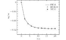
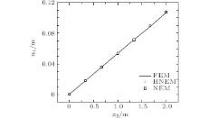
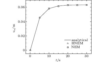
The radial displacements of nodes at x₂ = 0 when t = 30 s using the two models are given in Figs. 6 and 8. The displacements of node (1, 0) depending on time using the two models are shown in Figs. 7 and 9. From Figs. 6– 9, we can see that the results obtained by the HNEM have precision similar with that of the NEM and are in accord with the analytical solution.

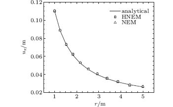	Figure Option View Download New Window
	Fig. 6. Radial displacements at x₂ = 0 obtained using the Maxwell model when t = 30 s.

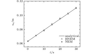	Figure Option View Download New Window
	Fig. 7. Time variation of radial displacement at point (1, 0) obtained using the Maxwell model.

	Figure Option View Download New Window
	Fig. 8. Radial displacements at x₂ = 0 obtained using the Kelvin model when t = 30 s.

	Figure Option View Download New Window
	Fig. 9. Time variation of radial displacement at point (1, 0) obtained using the Kelvin model.

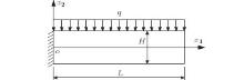
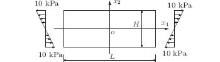
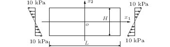
4.2. Cantilever beam with a distributed load

A cantilever beam with a distributed load is shown in Figs. 10. The length of the beam is L = 8 m and the width is H = 2 m. The distributed load is q = 30 kPa, and the volume deformation is elastic with E = 1.0× 10⁸ Pa, ν = 0.25. The rheological property of shear deformation satisfies the Kelvin model, and the corresponding parameters are G = 2× 10⁸ Pa and η = 6 × 10⁸ Pa · s. Regardless of the body force, the cantilever beam can be discussed in terms of a plane stress problem.

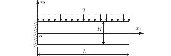	Figure Option View Download New Window
	Fig. 10. Cantilever beam with a distributed load.

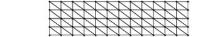
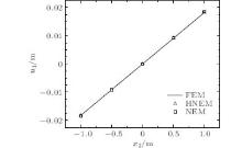
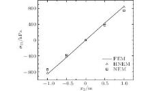
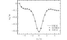
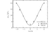
An array of 13 × 5 nodes is distributed on the beam, as shown in Figs. 11. The vertical and the horizontal displacements of the nodes at the left side of the cantilever beam are set as zero when calculated. Under the same nodal distribution, the numerical results obtained using the HNEM and the NEM are shown in Figs. 12– 15.From Figs. 12– 14, we can see that the nodal displacements obtained using the HNEM are in good agreement with those obtained using the NEM and the FEM; while the nodal stresses obtained using the HNEM are more precise than those from the NEM, as shown in Figs. 15.

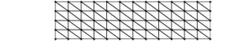	Figure Option View Download New Window
	Fig. 11. Nodal distribution and Delaunay triangles of the beam.

	Figure Option View Download New Window
	Fig. 12. Vertical displacements of nodes on the neutral axis of the beam when t = 20 s.

	Figure Option View Download New Window
	Fig. 13. Time variation of vertical displacement of point (8, 0).

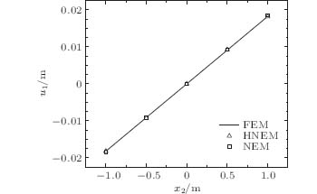	Figure Option View Download New Window
	Fig. 14. Horizontal displacements of nodes on the right edge of the beam when t = 20 s.

	Figure Option View Download New Window
	Fig. 15. Horizontal normal stress at x₁ = 2 m when t = 20 s.

4.3. Beam subjected to simple bending

Consider a beam subjected to simple bending, as shown in Figs. 16. The length is L = 10 m and the width is H = 4 m. The volume deformation is elastic and E = 1.0 × 10⁶ Pa, ν = 0.3. The three-parameter model is adopted to describe the rheological property of the shear deformation, and the parameters are G₁ = 5.0 × 10⁵ Pa, G₂ = 1.0 × 10⁶ Pa, and η = 2.0 × 10⁶ Pa · s. This example is discussed as a plane stress problem without considering the body force.

	Figure Option View Download New Window
	Fig. 16. Beam subjected to simple bending.

By taking advantage of the symmetry of the model, only a quarter of the model is considered in this analysis. At axes of x₁ and x₂, the horizontal displacements of the nodes are zero, and the vertical displacements of the nodes at the origin are set to zero for the restriction of rigid body displacements. As shown in Figs. 17, 13 × 7 nodes are arranged on a quarter of the model.

	Figure Option View Download New Window
	Fig. 17. Nodal distribution and Delaunay triangles in a quarter of the beam.

Under the same nodal distribution, the nodal displacements obtained using the HNEM and the NEM are described in Figs. 18– 20, and the nodal stresses are shown in Figs. 21. From Figs. 18– 20, we can see that the nodal displacements obtained using the HNEM are in good agreement with those obtained using the NEM and the FEM. The nodal stresses from the HNEM agree well with those from the FEM, while the precision of the nodal stresses is higher than that from the NEM, as shown in Figs. 21.

	Figure Option View Download New Window
	Fig. 18. Vertical displacements of nodes at x₂ = 0 when t = 30 s.

	Figure Option View Download New Window
	Fig. 19. Time variation of vertical displacement of node (5, 0).

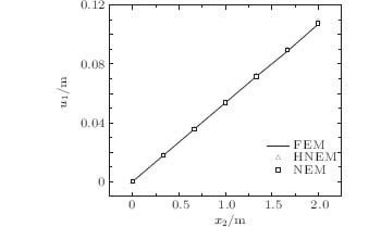	Figure Option View Download New Window
	Fig. 20. Horizontal displacements of nodes at x₁ = 5 m when t = 30 s.

	Figure Option View Download New Window
	Fig. 21. Horizontal normal stress at x₁ = 2.5 m when t = 30 s.

4.4. Plate with a central hole under an axial uniform tension

A plate with a central hole subjected to an axial uniform tension is shown in Figs. 22. The length of the plate is L = 10 m, the width is H = 4 m, and the radius of the hole is R = 1 m. The tensile load is q = 1 kPa, and the volume deformation is elastic with elasticity modulus E = 1.0× 10⁸ Pa, and Poisson ratio ν = 0.25. Using the three-parameter viscoelastic model, the corresponding parameters are G₁ = 8.0 × 10⁷ Pa, G₂ = 1.0 × 10⁸ Pa, and η = 2.0 × 10⁸ Pa · s. Regardless of the body force, the plate can be discussed as a plane stress problem.

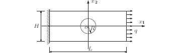	Figure Option View Download New Window
	Fig. 22. Plate with a central hole under an axial uniform tension.

There are 200 nodes distributed on the plate, as shown in Figs. 23. The vertical and the horizontal movements of the nodes at the left side of the plate are restricted in the procedure. The nodes near the hole are numerous so as to improve the calculation precision. The numerical results obtained by the HNEM and the NEM are shown in Figs. 24– 26. From Figs. 24 and 25, we can see that the nodal displacements solved by the HNEM fit well with those from the NEM and the FEM. In Figs. 26, it is shown that the nodal stresses gained by the HNEM are close to those by the FEM and have higher precision than those by the NEM.

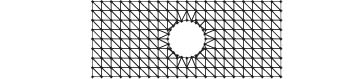	Figure Option View Download New Window
	Fig. 23. Nodal distribution and Delaunay triangles of the plate.

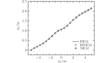	Figure Option View Download New Window
	Fig. 24. Horizontal displacements of the nodes at x₂ = 2 m when t = 30 s.

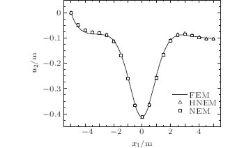	Figure Option View Download New Window
	Fig. 25. Vertical displacements of nodes at x₂ = 2 m when t = 30 s.

	Figure Option View Download New Window
	Fig. 26. Horizontal normal stresses of nodes at x₁ = − 2.5 m when t = 30 s.

5. Conclusion

In this paper, according to the properties of linear viscoelastic materials, the HNEM for linear viscoelastic materials under the creep condition is presented. The HNEM solves the problem that the nodal stresses cannot be obtained directly by the NEM.

Numerical examples show that the HNEM can obtain precise nodal displacements of linear viscoelastic materials, which illustrates the effectiveness of the method proposed in this paper. Under the same nodal distribution, the HNEM has a precision of nodal displacements similar to that of the NEM, while the precision of nodal stresses using the HNEM is higher than that using the NEM by the MLS approximation, which shows the superiority of this method.

Reference

View Option

1	Belytschko T, Lu Y Y and Gu L 1994 Int. J. Numer. Methods Eng. 37 229 [Cited within:1] [JCR: 2.056]
2	Wang J F, Sun F X and Cheng R J 2010 Chin. Phys. B 19 060201 [Cited within:1] [JCR: 1.148] [CJCR: 1.2429]
3	Cheng R J and Cheng Y M 2011 Chin. Phys. B 20 070206 [Cited within:1] [JCR: 1.148] [CJCR: 1.2429]
4	Zhang Z, Liew K M and Cheng Y M 2008 Engin. Anal. Bound. Elem. 32 100 [Cited within:1] [JCR: 1.596]
5	Zhang Z, Liew K M, Cheng Y M and Lee Y Y 2008 Engin. Anal. Bound. Elem. 32 241 [Cited within:1] [JCR: 1.596]
6	Zhang Z, Hao S Y, Liew K M and Cheng Y M 2013 Engin. Anal. Bound. Elem. 37 1576 [Cited within:1] [JCR: 1.596]
7	Zhang Z, Wang J F, Cheng Y M and Liew K M 2013 Sci. China-Phys. Mech. Astron. 56 1568 [Cited within:1]
8	Cheng Y M and Li J H 2005 Acta Phys. Sin. 54 4463(in Chinese) [Cited within:1] [JCR: 1.016] [CJCR: 1.691]
9	Wang J F and Cheng Y M 2012 Chin. Phys. B 21 120206 [Cited within:1] [JCR: 1.148] [CJCR: 1.2429]
10	Wang J F and Cheng Y M 2013 Chin. Phys. B 22 030208 [Cited within:1] [JCR: 1.148] [CJCR: 1.2429]
11	Peng M J, Liu P and Cheng Y M 2009 Int. J. Appl. Mech. 1 367 [Cited within:1] [JCR: 1.483]
12	Peng M J, Li D M and Cheng Y M 2011 Eng. Struct. 33 127 [Cited within:1] [JCR: 1.713]
13	Bai F N, Li D M, Wang J F and Cheng Y M 2012 Chin. Phys. B 21 020204 DOI:10.1088/1674-1056/21/2/020204 [Cited within:1] [JCR: 1.148] [CJCR: 1.2429]
14	Cheng Y M, Wang J F and Bai F N 2012 Chin. Phys. B 21 090203 DOI:10.1088/1674-1056/21/9/090203 [Cited within:1] [JCR: 1.148] [CJCR: 1.2429]
15	Li D M, Bai F N, Cheng Y M and Liew K M 2012 Comput. Meth. Appl. Mech. Eng. 233 236 1 DOI:10.1016/j.cma.2012.03.015 [Cited within:1]
16	Cheng Y M, Wang J F and Li R X 2012 Int. J. Appl. Mech. 4 1250042 DOI:10.1142/S1758825112500421 [Cited within:1] [JCR: 1.483]
17	Li D M, Liew K M and Cheng Y M 2014 Comput. Meth. Appl. Mech. Eng. 269 72 DOI:10.1016/j.cma.2013.10.018 [Cited within:1]
18	Ren H P and Cheng Y M 2011 Int. J. Appl. Mech. 3 735 DOI:10.1142/S1758825111001214 [Cited within:1] [JCR: 1.483]
19	Ren H P and Cheng Y M 2012 Eng. Anal. Bound. Elem. 36 873 DOI:10.1016/j.enganabound.2011.09.014 [Cited within:1] [JCR: 1.596]
20	Dai B D and Cheng Y M 2007 Acta Phys. Sin. 56 597 (in Chinese) [Cited within:1] [JCR: 1.016] [CJCR: 1.691]
21	Cheng R J and Cheng Y M 2007 Acta Phys. Sin. 56 5569 (in Chinese) [Cited within:1] [JCR: 1.016] [CJCR: 1.691]
22	Wang J F, Bai F N and Cheng Y M 2011 Chin. Phys. B 20 030206 DOI:10.1088/1674-1056/20/3/030206 [Cited within:1] [JCR: 1.148] [CJCR: 1.2429]
23	Atluri S N and Zhu T 1998 Comput. Mech. 22 117 DOI:10.1007/s004660050346 [Cited within:1] [JCR: 2.432]
24	Chen L and Cheng Y M 2008 Acta Phys. Sin. 57 1 (in Chinese) [Cited within:1] [JCR: 1.016] [CJCR: 1.691]
25	Chen L and Cheng Y M 2008 Acta Phys. Sin. 57 6047 (in Chinese) [Cited within:1] [JCR: 1.016] [CJCR: 1.691]
26	Chen L and Cheng Y M 2010 Chin. Phys. B 19 090204 DOI:10.1088/1674-1056/19/9/090204 [Cited within:1] [JCR: 1.148] [CJCR: 1.2429]
27	Chen L, Ma H P and Cheng Y M 2013 Chin. Phys. B 22 050202 DOI:10.1088/1674-1056/22/5/050202 [Cited within:1] [JCR: 1.148] [CJCR: 1.2429]
28	Weng Y J and Cheng Y M 2013 Chin. Phys. B 22 090204 DOI:10.1088/1674-1056/22/9/090204 [Cited within:1] [JCR: 1.148] [CJCR: 1.2429]
29	Li S C, Cheng Y M and Li S C 2006 Acta Phys. Sin. 55 4760 (in Chinese) [Cited within:1] [JCR: 1.016] [CJCR: 1.691]
30	Gao H F and Cheng Y M 2010 Int. J. Comput. Methods 7 55 DOI:10.1142/S0219876210002064 [Cited within:1] [JCR: 0.481]
31	Cheng Y M and Chen M J 2003 Acta Mech. Sin. 35 181 (in Chinese) DOI:10.6052/0459-1879-2003-2-2002-036 [Cited within:1] [CJCR: 0.558]
32	Cheng Y M and Peng M J 2005 Sci. Chin. Ser. G: Phys. Mech. Astron 48 641 DOI:10.1007/BF02687411 [Cited within:1]
33	Kitipornchai S, Liew K M and Cheng Y M 2005 Comput. Mech. 36 13 DOI:10.1007/s00466-004-0638-1 [Cited within:1] [JCR: 2.432]
34	Liew K M, Cheng Y M and Kitipornchai S 2005 Int. J. Numer. Methods Eng. 64 1610 [Cited within:1] [JCR: 2.056]
35	Liew K M, Cheng Y M and Kitipornchai S 2006 Int. J. Numer. Methods Eng. 65 1310 [Cited within:1] [JCR: 2.056]
36	Qin Y X and Cheng Y M 2006 Acta Phys. Sin. 55 3215 (in Chinese) [Cited within:1] [JCR: 1.016] [CJCR: 1.691]
37	Liew K M, Cheng Y M and Kitipornchai S 2007 Int. J. Solids Struct. 44 4220 DOI:10.1016/j.ijsolstr.2006.11.018 [Cited within:1] [JCR: 1.871]
38	Cheng Y M, Liew K M and Kitipornchai S 2009 Int. J. Numer. Methods Eng. 78 1258 DOI:10.1002/nme.v78:10 [Cited within:1] [JCR: 2.056]
39	Liew K M and Cheng Y M 2009 Comput. Meth. Appl. Mech. Eng. 198 3925 DOI:10.1016/j.cma.2009.08.020 [Cited within:1]
40	Peng M J and Cheng Y M 2009 Eng. Anal. Bound. Elem. 33 77 DOI:10.1016/j.enganabound.2008.03.005 [Cited within:1] [JCR: 1.596]
41	Ren H P, Cheng Y M and Zhang W 2009 Chin. Phys. B 18 4065 DOI:10.1088/1674-1056/18/10/002 [Cited within:1] [JCR: 1.148] [CJCR: 1.2429]
42	Ren H P, Cheng Y M and Zhang W 2010 Sci. China-Phys. Mech. Astron. 53 758 DOI:10.1007/s11433-010-0159-1 [Cited within:1]
43	Wang J F, Sun F X and Cheng Y M 2012 Chin. Phys. B 21 090204 DOI:10.1088/1674-1056/21/9/090204 [Cited within:1] [JCR: 1.148] [CJCR: 1.2429]
44	Wang J F, Wang J F, Sun F X and Cheng Y M 2013 Int. J. Comput. Methods 10 1350043 DOI:10.1142/S0219876213500436 [Cited within:1] [JCR: 0.481]
45	Braun J and Sambridge M 1995 Nature 376 655 DOI:10.1038/376655a0 [Cited within:1] [JCR: 38.597]
46	Sukumar N, Moran B and Belytschko T 1998 Int. J. Numer. Methods Eng. 43 839 [Cited within:1] [JCR: 2.056]
47	Bueche D, Sukumar N and Moran B 2000 Comput. Mech. 25 207 DOI:10.1007/s004660050470 [Cited within:1] [JCR: 2.432]
48	Cueto E, Calvo B and Doblare M 2002 Int. J. Numer. Methods Eng. 54 871 [Cited within:1] [JCR: 2.056]
49	Martínez M, Cueto E, Doblaré M and Chinesta F 2003 J. Non-Newton. Fluid Mech. 115 51 DOI:10.1016/S0377-0257(03)00171-X [Cited within:1]
50	Calvo B, Martinez M A and Doblaré M 2005 Int. J. Numer. Methods Eng. 62 159 [Cited within:1] [JCR: 2.056]
51	Daneshmand F and Niroomand i S 2007 Eng. Comput. 24 269 DOI:10.1108/02644400710735034 [Cited within:1]
52	Daneshmand F, Javanmard S S, Liaghat T, Moshksar M M and Adamowski J F 2010 Can. J. Civ. Eng. 37 1550 DOI:10.1139/L10-087 [Cited within:1]
53	Shahrokhabadi S, Toufigh M M and Gholizadeh R 2010GeoShanghai International Conference-Geoenvironmental Engineering and GeotechnicsJune 3–5, 2010Shanghai, China 245 DOI:10.1061/41105(378)34 [Cited within:1]
54	Cho J R, Lee H W and Yoo W S 2013 Comput. Meth. Appl. Mech. Eng. 256 17 DOI:10.1016/j.cma.2012.12.015 [Cited within:1]
55	Sibson R 1980Mathematical Proceedings of the Cambridge Philosophical SocietyJanuary, 1980Cambridge, England 151 DOI:10.1017/S0305004100056589 [Cited within:1]
56	Farin G 1990 Comput. Aided Geom. Des. 7 281 DOI:10.1016/0167-8396(90)90036-Q [Cited within:1]
57	Brown J L 1994An international conference on curves and surfaces on Wavelets, images, and surface fitting1994Chamonix-Mont-Blanc, France 67 [Cited within:1]
58	Tabbara M, Blacker T and Belytschko T 1994 Comput. Methods Appl. Mech. Engin. 117 211 DOI:10.1016/0045-7825(94)90084-1 [Cited within:1]
59	Dong Y, Ma Y Q and Feng W 2012 Acta Mech. Sin. 44 568 (in Chinese) DOI:10.6052/0459-1879-2012-3-20120313 [Cited within:1] [CJCR: 0.558]
60	Ma Y Q, Dong Y, Zhou Y K and Feng W 2014 Math. Probl. Eng. 2014 9 DOI:10.1155/2014/979216 [Cited within:1] [JCR: 1.383]
61	Belikov V, Ivanov V, Kontorovich V, Korytnik S and Semenov A Y 1997 Comput. Math. Math. Phys. 37 9 [Cited within:2] [JCR: 0.408]
62	Sukumar N 2001Proceedings of the first MIT Conference on Fluid and Solid MechanicsJune 12–14 2001Cambridge, USA 1665 [Cited within:3]
63	Tian Z S and Pian T H 2011 Multivariable Variation Principle and Multivariable Finite Element Method 1 1 Beijing Science Press (in Chinese) [Cited within:1]
64	Pian T H and Chen D P 1982 Int. J. Numer. Methods Eng. 18 1679 [Cited within:1] [JCR: 2.056]
65	Peng M J and Xu Z H 2006 Sci. Chin. Ser. G: Phys. Mech. Astron. 49 671 DOI:10.1007/s11433-006-2003-1 [Cited within:1]
66	Flügge W 1975 Viscoelasticity2nd New York Springer-Verlag 1 DOI:10.1007/978-3-662-02276-4 [Cited within:3]
67	Yang H T and Liu Y 2003 Int. J. Solids Struct. 40 701 DOI:10.1016/S0020-7683(02)00614-5 [Cited within:1] [JCR: 1.871]
68	Sladek J, Sladek V and Zhang C 2005 Engin. Anal. Bound. Elem. 29 597 DOI:10.1016/j.enganabound.2005.01.011 [Cited within:1] [JCR: 1.596]
69	Sladek J, Sladek V, Zhang C and Schanz M 2006 Comput. Mech. 37 279 DOI:10.1007/s00466-005-0715-0 [Cited within:1] [JCR: 2.432]
70	Guan Y J, Zhao G Q, Wu X and Lu P 2007 J. Mater. Process. Technol. 187–188 412 DOI:10.1016/j.jmatprotec.2006.11.075 [Cited within:1]
71	Canelas A and Sensale B 2010 Eng. Anal. Bound. Elem. 34 845 DOI:10.1016/j.enganabound.2010.05.010 [Cited within:1] [JCR: 1.596]
72	Cheng Y M, Li R X and Peng M J 2012 Chin. Phys. B 21 090205 DOI:10.1088/1674-1056/21/9/090205 [Cited within:1] [JCR: 1.148] [CJCR: 1.2429]
73	Peng M J, Li R X and Cheng Y M 2014 Engin. Anal. Bound. Elem. 40 104 DOI:10.1016/j.enganabound.2013.11.018 [Cited within:1] [JCR: 1.596]
74	Lawson C L 1977 Mathematical Software III 3nd edn. New York Academic Press 161 194 [Cited within:1]

1994

2.056

0.0

... ^[1] In addition to the EFG method,^[2,3] there are many other meshless methods, such as the improved element-free Galerkin method,^{[4#cod#x2013 ...}

2010

1.148

1.2429

... ^[1] In addition to the EFG method,^[2,3] there are many other meshless methods, such as the improved element-free Galerkin method,^{[4#cod#x2013 ...}

2011

1.148

1.2429

... ^[1] In addition to the EFG method,^[2,3] there are many other meshless methods, such as the improved element-free Galerkin method,^{[4#cod#x2013 ...}

2008

1.596

0.0

Zhang

, Liew

K M

and Cheng

Y M

2008 Engin. Anal. Bound. Elem. 32 100

Abstract In this paper, the element-free Galerkin (EFG) method and improved moving least-squares (IMLS) approximation are combined. An improved FEG (IEFG) method for two-dimensional elasticity is discussed, and the coupling of the IEFG method and the boundary element method (BEM) is presented. In the IMLS approximation, an orthogonal function system with a weight function is used as the basis function. The IMLS approximation has greater computational efficiency and precision than the existing moving least-squares (MLS) approximation, and does not lead to an ill-conditioned system of equations. There are fewer coefficients in the IMLS approximation than in the MLS approximation, and in the IEFG method that is formed with the IMLS approximation fewer nodes are selected in the entire domain than are selected using the conventional EFG method. Hence, the IEFG method should result in a higher computing speed. Based on the IMLS approximation and the IEFG method, a direct coupling of the IEFG method and the BEM is discussed for two-dimensional elasticity problems, and the corresponding formulae of the coupled method are obtained. The coupled method does not need a new sub-domain between the IEFG method and the BEM sub-domains. Selected numerical examples are solved using the coupled method.

... ^[1] In addition to the EFG method,^[2,3] there are many other meshless methods, such as the improved element-free Galerkin method,^{[4#cod#x2013 ...}

2008

1.596

0.0

Zhang

, Liew

K M

, Cheng

Y M

and Lee

Y Y

2008 Engin. Anal. Bound. Elem. 32 241

Abstract This paper presents an improved moving least-squares (IMLS) approximation in which the orthogonal function system with a weight function is used as the basis function. The IMLS approximation has greater computational efficiency and precision than the existing moving least-squares (MLS) approximation, and does not lead to an ill-conditioned system of equations. By combining the element-free Galerkin (EFG) method and the IMLS approximation, an improved element-free Galerkin (IEFG) method for two-dimensional elasticity is derived. There are fewer coefficients in the IMLS approximation than in the MLS approximation, and in the IEFG method that is formed with the IMLS approximation fewer nodes are selected in the entire domain than are selected in the conventional EFG method. Hence, the IEFG method should result in a higher computing speed. For two-dimensional fracture problems, the enriched basis function is used at the tip of the crack to give an enriched IEFG method. When the enriched IEFG method is used, the singularity of the stresses at the tip of the crack can be shown better than that in the IEFG method. To provide a demonstration, numerical examples are solved using the IEFG method and the enriched IEFG method.

2013

1.596

0.0

Zhang

, Hao

S Y

, Liew

K M

and Cheng

Y M

2013 Engin. Anal. Bound. Elem. 37 1576

In this paper, we derive an improved element-free Galerkin (IEFG) method for two-dimensional linear elastodynamics by employing the improved moving least-squares (IMLS) approximation. In comparison with the conventional moving least-squares (MLS) approximation function, the algebraic equation system in IMLS approximation is well-conditioned. It can be solved without having to derive the inverse matrix. Thus the IEFG method may result in a higher computing speed. In the IEFG method for two-dimensional linear elastodynamics, we employed the Galerkin weak form to derive the discretized system equations, and the Newmark time integration method for the time history analyses. In the modeling process, the penalty method is used to impose the essential boundary conditions to obtain the corresponding formulae of the IEFG method for two-dimensional elastodynamics. The numerical studies illustrated that the IEFG method is efficient by comparing it with the analytical method and the finite element method. (C) 2013 Elsevier Ltd. All rights reserved.

Zhang, Zan 1 ;Hao, S. Y. 2 ;Liew, K. M. 3 ;Cheng, Y. M. 4 ;

2013

0.0

... 7] the complex variable meshless method,^{[8#cod#x2013 ...}

2005

1.016

1.691

Cheng

Y M

and Li

J H

2005 Acta Phys. Sin. 54 4463(in Chinese)

The moving least-square approximation with complex variables (MLSCV) is developed on the basis of moving least-square approximation. The advantages of MLSCV are that the approximation function of a 2-D problem is formed with 1-D basis function, and the meshless method obtained has greater computational efficiency. A meshless method with complex variables for 2-D elasticity is then presented using MLSCV, and the formulae of the meshless method with complex variables are obtained. Compared with the conventional meshless method, the meshless method with complex variables introduced in this paper has greater precision and computational efficiency. Some examples are given.

(1)上海大学上海市应用数学和力学研究所，上海 200072; (2)西安理工大学水利水电学院，西安 710048

在移动最小二乘法的基础上，提出了复变量移动最小二乘法.复变量移动最小二乘法的优点是采用一维基函数建立二维问题的逼近函数，所形成的无网格方法计算量小.然后，将复变量移动最小二乘法应用于弹性力学的无网格方法，提出了复变量无网格方法，推导了复变量无网格方法的公式.与传统的无网格方法相比，复变量无网格方法具有计算量小、精度高的优点.最后给出了数值算例.

... 7] the complex variable meshless method,^{[8#cod#x2013 ...}

2012

1.148

1.2429

2013

1.148

1.2429

Wang

J F

and Cheng

Y M

2013 Chin. Phys. B 22

030208

Effects of an ultra-strong magnetic field on electron capture rates for Co-55 are analyzed in the nuclear shell model and under the Landau energy levels quantized approximation in the ultra-strong magnetic field, and the electron capture rates on 10 abundant iron group nuclei at the surface of a magnetar are given. The results show that electron capture rates on Co-55 are increased greatly in the ultra-strong magnetic field, by about 3 orders of magnitude generally. These conclusions play an important role in future study of the evolution of magnetars.

Du Jun 1 ;Li Ping-Ping 1 ;Luo Xia 1,2 ;

Effects of ultra-strong magnetic field on electron capture rates for 55 Co are analyzed in the nuclear shell model and under the Landau energy levels quantized approximation in the ultra-strong magnetic field, and the electron capture rates on 10 abundant iron group nuclei at the surface of magnetar are given. The results show that electron capture rates on 55 Co are increased greatly in the ultra-strong magnetic field, by about 3 orders of magnitude generally. These conclusions play an important role in future studying the evolution of magnetar.

... 10] the complex variable element-free Galerkin (CVEFG) method,^{[11#cod#x2013 ...}

2009

1.483

0.0

... 10] the complex variable element-free Galerkin (CVEFG) method,^{[11#cod#x2013 ...}

2011

1.713

0.0

Peng

M J

, Li

D M

and Cheng

Y M

2011 Eng. Struct. 33 127

Abstract Based on the complex variable moving least-squares (CVMLS) approximation and element-free Galerkin (EFG) method, the complex variable element-free Galerkin (CVEFG) method for two-dimensional elasto-plasticity problems is presented in this paper. The CVMLS approximation is an approximation method for a vector function. Under the same node distribution the meshless method based on the CVMLS approximation has higher precision than the one based on the moving least-squares (MLS) approximation. For two-dimensional elasto-plasticity problems, the Galerkin weak form is employed to obtain the equations system, and the penalty method is used to apply the essential boundary conditions, then the corresponding formulae of the CVEFG method for two-dimensional elasto-plasticity problems are obtained. Compared with the EFG method, the CVEFG method can obtain greater precision. For the purposes of demonstration, some selected numerical examples are solved using the CVEFG method.

2012

1.148

1.2429

2012

1.148

1.2429

2012

0.0

2012

1.483

0.0

2014

0.0

... 17] the interpolating element-free Galerkin (IEFG) method,^{[18, 19]} the radial basis function (RBF) method,^[20] the finite point method (FPM),^{[21, 22]} the meshless local Petrov#cod#x2013 ...

2011

1.483

0.0

2012

1.596

0.0

2007

1.016

1.691

Dai

B D

and Cheng

Y M

2007 Acta Phys. Sin. 56 597 (in Chinese)

Combining the interpolation function, which has the delta function property and is constructed on the basis of radial basis functions and polynomial functions, using the local boundary integral equation method (LBIE), the local boundary integral equation method based on radial basis functions is presented for potential problem in this paper. The corresponding discrete equations are obtained. Comparing with the other meshless boundary integral equation methods, the present method has simpler numerical procedures, lower computation cost and higher accuracy. In addition, the essential boundary conditions can be implemented directly. Some numerical results to show the efficiency of the present method are given.

(1)上海大学上海市应用数学和力学研究所，上海 200072; (2)上海大学上海市应用数学和力学研究所，上海 200072；太原科技大学工程力学系，太原 030024

将基于径向基函数构造的具有插值特性的近似函数和局部边界积分方程方法相结合，建立了求解势问题的径向基函数——局部边界积分方程方法，推导了相应离散方程.与其他边界积分方程的无网格方法相比，本文方法具有数值实现过程简单、计算量小、精度高的优点，并可直接施加边界条件.最后通过算例说明了该方法的有效性.

2007

1.016

1.691

Cheng

R J

and Cheng

Y M

2007 Acta Phys. Sin. 56 5569 (in Chinese)

In this paper, the finite point method is used to obtain the solution of a one-d imensional inverse heat conduction problem with a source parameter, and the corr esponding discrete equations are obtained. Compared with the numerical methods b ased on mesh, the finite point method only needs the scattered nodes instead of meshing the domain of the problem. The finite point method is a meshless method in which the moving least-square approximation is used to form the meshless appr oximation functions. And the collocation method is used to discretize the govern ing partial differential equations. The finite point method has the advantages o f simpler numerical procedures, lower computation cost and arbitrary nodes. The result of a numerical example is presented to show the method is effective.

(1)上海大学上海市应用数学和力学研究所，上海 200072; (2)上海大学上海市应用数学和力学研究所，上海 200072;安徽师范大学数学系，芜湖 241000

利用无网格有限点法求带有源参数的一维热传导反问题，推导了相应的离散方程.与其他基于网格的方法相比，有限点法采用移动最小二乘法构造形函数，只需要节点信息，不需要划分网格，用配点法离散求解方程，可以直接施加边界条件，不需要在区域内部求积分，减小了计算量.用有限点法求解热传导反问题具有数值实现简单、计算量小、可以任意布置节点等优点.最后通过算例验证了该方法的有效性.

2011

1.148

1.2429

1998

2.432

0.0

... Galerkin (MLPG) method,^[23] the reproducing kernel particle method (RKPM),^{[24#cod#x2013 ...}

2008

1.016

1.691

... Galerkin (MLPG) method,^[23] the reproducing kernel particle method (RKPM),^{[24#cod#x2013 ...}

2008

1.016

1.691

Chen

and Cheng

Y M

2008 Acta Phys. Sin. 57 6047 (in Chinese)

On the basis of reproducing kernel particle method(RKPM), the complex variable reproducing kernel particle method (CVRKPM) is discussed. The advantage of the CVRKPM is that the correction function of a 2-D problem is formed with 1-D basis function when the shape function is obtained. Then, we apply the complex variable method to two-dimensional transient heat conduction problems. In combination with the Galerkin weak form of transient heat conduction problems, the penalty method is employed to enforce the essential boundary conditions, the CVRKPM for transient heat conduction problems is investigated and the corresponding formulae are obtained. Compared with the conventional RKPM, the CVRKPM introduced in this paper has a higher precision and a lower computation cost. Some examples given in this paper verify the effectivity of the proposed method.

(1)上海大学上海市应用数学和力学研究所，上海 200072; (2)上海大学上海市应用数学和力学研究所，上海 200072；长安大学理学院工程力学系，西安 710064

在重构核粒子法的基础上，引入复变量，讨论了复变量重构核粒子法.复变量重构核粒子法的优点是在构造形函数时采用一维基函数建立二维问题的修正函数.然后，将复变量重构核粒子法应用于瞬态热传导问题的求解，结合瞬态热传导问题的Galerkin积分弱形式，采用罚函数法引入本质边界条件，建立了瞬态热传导问题的复变量重构核粒子法，推导了相应的计算公式.与传统的重构核粒子法相比，复变量重构核粒子法具有计算量小、精度高的优点.最后通过数值算例证明了该方法的有效性.

2010

1.148

1.2429

2013

1.148

1.2429

Chen

, Ma

H P

and Cheng

Y M

2013 Chin. Phys. B 22

050202

DOI:10.1088/1674-1056/22/5/050202

Du Jun 1 ;Li Ping-Ping 1 ;Luo Xia 1,2 ;

2013

1.148

1.2429

Weng

Y J

and Cheng

Y M

2013 Chin. Phys. B 22

090204

DOI:10.1088/1674-1056/22/9/090204

Du Jun 1 ;Li Ping-Ping 1 ;Luo Xia 1,2 ;

... 28] the meshless manifold method,^{[29, 30]} the boundary element-free method (BEFM),^{[31#cod#x2013 ...}

2006

1.016

1.691

S C

, Cheng

Y M

and Li

S C

2006 Acta Phys. Sin. 55 4760 (in Chinese)

In the paper, the meshless manifold method (MMM) is utilized to analyze transient deformations in dynamic fracture. The MMM is based on the partition of unity method and the finite coverage approximation which provides a unified framework for solving problems involving both continuums and dis-continuums. The method can treat crack problem easily because the shape function is not affected by the discontinuity in the domain. For localization problems at the tip of the discontinuity, these shape functions are more effective than those used in other numerical methods. The method avoids the disadvantages of other meshless methods in which the tip of a discontinuous crack is not considered. In meshless manifold method, the finite coverage approximation is used to construct the shape functions that overcome influences of the interior discontinuities in the displacement. Consequently, the meshless manifold method has some advantages in solving the discontinuity problems when the discontinuities are complex. When the dynamic fracture mechanics is analyzed by the MMM, the weak formulation of the partial differential equation for elastic dynamics is derived from the method of weighted residuals (MWR). The discrete space of the domain is used for the MMM. The Newmark family of methods is used for the time integration scheme. At last, the validity and accuracy of the MMM are illustrated by two numerical examples of which the numerical results agree with the analytical solution.

(1)山东大学土建与水利学院，济南 250061; (2)上海大学上海市应用数学和力学研究所，上海 200072

运用无网格流形方法求解动态断裂力学问题.该方法利用单位分解法和有限覆盖技术建立形函数，形函数的建立不受域内不连续的影响，可较好地求解裂纹问题.对于局部化问题，该方法的形函数构造较其他方法更为有效，避免了其他方法在建立试函数时没有考虑不连续尖端的缺点.由于采用有限覆盖技术建立试函数，该方法克服了不连续对试函数的影响，尤其当不连续变得复杂时，更能显示该方法在处理不连续方面的优点.在求解动态断裂力学问题时，弹性动力学积分弱形式的推导采用加权残数法，空间离散采用基于单位分解法的无网格流形方法，时间离散主要采用Newmark法.最后给出两个数值算例，将计算结果与解析解对比，说明该方法的正确性和可行性.

... 28] the meshless manifold method,^{[29, 30]} the boundary element-free method (BEFM),^{[31#cod#x2013 ...}

2010

0.481

0.0

... 28] the meshless manifold method,^{[29, 30]} the boundary element-free method (BEFM),^{[31#cod#x2013 ...}

2003

0.0

0.558

... 28] the meshless manifold method,^{[29, 30]} the boundary element-free method (BEFM),^{[31#cod#x2013 ...}

2005

0.0

2005

2.432

0.0

2005

2.056

0.0

2006

2.056

0.0

2006

1.016

1.691

Qin

Y X

and Cheng

Y M

2006 Acta Phys. Sin. 55 3215 (in Chinese)

By combining the reproducing kernel particle method (RKPM) and boundary integral equation method for elasticity, the reproducing kernel particle boundary element-free (RKP-BEF) method is presented in this paper. Formulae for the RKP-BEF method are derived. The discrete boundary integral equations of the RKP-BEF method are established by considering the numerical integral schemes and the treatment of singular integrals, and the formulae of the displacement and stress of inner points for the RKP-BEF method are given. The RKP-BEF method has a higher precision as the smoothness of the shape function of RKP method is the same as that of the kernel function, and the values of polynomials at interpolating points can be exactly reconstructed. Numerical examples are given for verifying the effectiveness and correctness of the RKP-BEF method presented in this paper.

(1)上海大学上海市应用数学和力学研究所，上海 200072; (2)上海大学上海市应用数学和力学研究所，上海 200072;太原科技大学，太原 030024

将重构核粒子法(RKPM)和边界积分方程方法结合，提出了一种新的边界积分方程无网格方法——重构核粒子边界无单元法(RKP-BEFM).对弹性力学问题，推导了其重构核粒子边界无单元法的公式，研究其数值积分方案，建立了重构核粒子边界无单元法离散化边界积分方程，并推导了重构核粒子边界无单元法的内点位移和应力积分公式.重构核粒子法形成的形函数具有重构核函数的光滑性，且能再现多项式在插值点的精确值，所以本方法具有更高的精度.最后给出了数值算例，验证了本方法的有效性和正确性.

2007

1.871

0.0

2009

2.056

0.0

2009

0.0

2009

1.596

0.0

Peng

M J

and Cheng

Y M

2009 Eng. Anal. Bound. Elem. 33 77 DOI:10.1016/j.enganabound.2008.03.005

Abstract Combining the boundary integral equation (BIE) method and improved moving least-squares (IMLS) approximation, a direct meshless BIE method, which is called the boundary element-free method (BEFM), for two-dimensional potential problems is discussed in this paper. In the IMLS approximation, the weighted orthogonal functions are used as the basis functions; then the algebra equation system is not ill-conditioned and can be solved without obtaining the inverse matrix. Based on the IMLS approximation and the BIE for two-dimensional potential problems, the formulae of the BEFM are given. The BEFM is a direct numerical method in which the basic unknown quantity is the real solution of the nodal variables, and the boundary conditions can be applied directly and easily; thus, it gives a greater computational precision. Some numerical examples are presented to demonstrate the method.

... 40] and the improved boundary element-free method (IBEFM) ...

2009

1.148

1.2429

Ren

H P

, Cheng

Y M

and Zhang

2009 Chin. Phys. B 18 4065 DOI:10.1088/1674-1056/18/10/002

The interpolating moving least-squares (IMLS) method is discussedfirst in this paper. And the formulae of the IMLS method obtained byLancaster are revised. Then on the basis of the boundaryelement-free method (BEFM), combining the boundary integral equation(BIE) method with the IMLS method, the improved boundaryelement-free method (IBEFM) for two-dimensional potential problemsis presented, and the corresponding formulae of the IBEFM areobtained. In the BEFM, boundary conditions are applied directly, butthe shape function in the MLS does not satisfy the property ofthe Kronecker δ function. This is a problem of the BEFM, andmust be solved theoretically. In the IMLS method, when the shape functionsatisfies the property of the Kronecker δ function, then theboundary conditions, in the meshless method based on the IMLSmethod, can be applied directly. Then the IBEFM, based on the IMLSmethod, is a direct meshless boundary integral equation method inwhich the basic unknown quantity is the real solution of the nodalvariables, and the boundary conditions can be applied directly andeasily, thus it gives a greater computational precision. Somenumerical examples are presented to demonstrate the method.

School of Computer Engineering and Science, Shanghai University, Shanghai 200072, China

... ^{[41#cod#x2013 ...}

2010

0.0

2012

1.148

1.2429

2013

0.481

0.0

Wang

J F

, Wang

J F

, Sun

F X

and Cheng

Y M

2013 Int. J. Comput. Methods 10

1350043

DOI:10.1142/S0219876213500436

An effective algorithm for the finite-horizon linear quadratic continuous terminal control is proposed. It is the combination of existing continuous soft and hard terminal control. We apply the algorithm to the automatic landing control of OH-6A helicopters. Numerical demonstration shows that, whether noise exists or not, the algorithm has less computation time and less feedback gains than existing hard terminal control while generally achieving the same terminal accuracy. The optimization problem which represents the hard terminal control can be addressed by sweep method and transit matrix method. It is also discovered that transit matrix method is a crucial point for improving terminal accuracy.

Xia, X. 1 ;Xu, Z. 1 ;

... 44] ...

1995

38.597

0.0

... ^[45] this method has been successfully applied in solid mechanics and fluid mechanics ...

1998

2.056

0.0

... ^[46] successfully solved partial differential equations of the elliptic type in solid mechanics by using this method ...

2000

2.432

0.0

... ^[47] researched the NEM for elastokinetics problems ...

2002

2.056

0.0

... ^[48] extended the NEM based on the concept of an #cod#x0061 ...

2003

0.0

... ^[49] applied the NEM in the analysis of fluids ...

2005

2.056

0.0

... ^[50] studied the NEM for large deformation problems ...

2007

0.0

... ^[51] Daneshmand et al ...

2010

0.0

... ^[52] used the NEM to calculate the two-dimensional flow under sluice gates ...

2010

0.0

... ^[53] used the NEM to analyze seepage problems of underground water ...

2013

0.0

... ^[54] ...

1980

0.0

... )except at the nodes where they are C⁰,^{[55#cod#x2013 ...}

1990

0.0

1994

0.0

... 57] we cannot obtain the nodal stresses ...

1994

0.0

... ^[58] Except for this method, the hybrid natural element method (HNEM) can also obtain the nodal stresses, which has been successfully applied in elasticity problems and elastoplasticity problems ...

2012

0.0

0.558

... ^[59,60] The HNEM adopts displacement interpolation and stress interpolation respectively using natural neighbor interpolation,^[61,62] and the corresponding formulae are obtained according to the Hellinger#cod#x2013 ...

2014

1.383

0.0

1997

0.408

0.0

... The shape functions for the HNEMThe natural neighbor interpolation (NNI)^[61,62] in the NEM is adopted to construct the shape functions for the HNEM ...

2001

0.0

... The shape functions for the HNEMThe natural neighbor interpolation (NNI)^[61,62] in the NEM is adopted to construct the shape functions for the HNEM ...

... ^[62] ...

2011

0.0

... ^[63,64] ...

1982

2.056

0.0

... ^[63,64] ...

2006

0.0

... ^[65] The constitutive relationship of viscoelastic materials correlates with time ...

1975

0.0

... ^[66] The solutions of complex viscoelastic problems in engineering mainly rely on numerical calculations, for which the meshless methods have been widely used ...

... In the polar coordinates, the analytical solution of the radial displacement of a Maxwell material is given by^[66] ...

... In the polar coordinates, the analytical solution of the radial displacement of a Kelvin material is given by^[66](67)

2003

1.871

0.0

Yang

H T

and Liu

2003 Int. J. Solids Struct. 40 701 DOI:10.1016/S0020-7683(02)00614-5

Abstract In this paper, element free Galerkin (EFG) method is combined with a precise algorithm in the time domain for solving viscoelasticity problems. By expanding variables at discretized time intervals, an initial boundary value problem is converted into a series of recurrent boundary value problems which can be conveniently solved by EFG/EFG-FE with a self-adaptive computing process. There is no requirement of iteration for the solution of non-linear cases. Satisfactory numerical results are obtained for both static and dynamical viscoelasticity problems.

... ^[67] Using the meshless local Petrov#cod#x2013 ...

2005

1.596

0.0

Sladek

, Sladek

and Zhang

2005 Engin. Anal. Bound. Elem. 29 597 DOI:10.1016/j.enganabound.2005.01.011

Abstract A meshless method based on the local Petrov–Galerkin approach is proposed for stress analysis in two-dimensional (2D), anisotropic and linear elastic/viscoelastic solids with continuously varying material properties. The correspondence principle is applied for non-homogeneous, anisotropic and linear viscoelastic solids where the relaxation moduli are separable in space and time. The inertial dynamic term in the governing equations is considered too. A unit step function is used as the test functions in the local weak-form. It leads to local boundary integral equations (LBIEs). The analyzed domain is divided into small subdomains with a circular shape. The moving least squares (MLS) method is adopted for approximating the physical quantities in the LBIEs. For time-dependent problems, the Laplace-transform technique is utilized. Several numerical examples are given to verify the accuracy and the efficiency of the proposed method.

... ^{[68, 69]} analyzed anisotropic and linear viscoelastic solids, and discussed quasistatic and transient dynamic problems in two-dimensional linear viscoelastic media ...

2006

2.432

0.0

Sladek

, Sladek

, Zhang

and Schanz

2006 Comput. Mech. 37 279 DOI:10.1007/s00466-005-0715-0

A meshless method based on the local Petrov-Galerkin approach is proposed for the solution of quasi-static and transient dynamic problems in two-dimensional (2-D) nonhomogeneous linear viscoelastic media. A unit step function is used as the test functions in the local weak form. It is leading to local boundary integral equations (LBIEs) involving only a domain-integral in the case of transient dynamic problems. The correspondence principle is applied to such nonhomogeneous linear viscoelastic solids where relaxation moduli are separable in space and time variables. Then, the LBIEs are formulated for the Laplace-transformed viscoelastic problem. The analyzed domain is covered by small subdomains with a simple geometry such as circles in 2-D problems. The moving least squares (MLS) method is used for approximation of physical quantities in LBIEs.

1.Institute of Construction and Architecture, Slovak Academy of Sciences, 84503 Bratislava, Slovakia 2.Department of Civil Engineering, University of Siegen, D-57068 Siegen, Germany 3.Institute of Applied Mechanics, Graz University of Technology, A-8010 Graz, Austria

... ^{[68, 69]} analyzed anisotropic and linear viscoelastic solids, and discussed quasistatic and transient dynamic problems in two-dimensional linear viscoelastic media ...

2007

0.0

... ^[70] Canelas and Sensale studied a boundary knot method for harmonic elastic and viscoelastic problems ...

2010

1.596

0.0

Canelas

and Sensale

2010 Eng. Anal. Bound. Elem. 34 845 DOI:10.1016/j.enganabound.2010.05.010

Abstract The boundary knot method is a promising meshfree, integration-free, boundary-type technique for the solution of partial differential equations. It looks for an approximation of the solution in the linear span of a set of specialized radial basis functions that satisfy the governing equation of the problem. The boundary conditions are taken into account through the collocation technique. The specialized radial basis function for harmonic elastic and viscoelastic problems is derived, and a boundary knot method for the solution of these problems is proposed. The completeness issue regarding the proposed set of radial basis functions is discussed, and a formal proof of incompleteness for the circular ring problem is presented. In order to address the numerical performance of the proposed method, some numerical examples considering simple and complex domains are solved.

... ^[71] A complex variable element-free Galerkin method for linear viscoelasticity problems under the creep condition was analyzed by Cheng et al ...

2012

1.148

1.2429

... ^[72] Three-dimensional viscoelasticity problems were analyzed via the improved element-free Galerkin method by Peng et al ...

2014

1.596

0.0

... ^[73] ...

1977

0.0

... ^[74] The natural neighbor nodes of x are 1, 5, 6, and 7, as shown in Fig ...