Due to the important role that the nonlinear theory plays in mathematics, physics, chemistry, biology, communications, astrophysics, and geophysics, much endeavor has been devoted to finding important and significant properties of different types of nonlinear equations, among which, the study on the integrable systems occupies the most important place. The integrable systems are introduced by scientists with some ideal conditions to describe complex nonlinear phenomena, such as the Korteweg– de Vries (KdV) equation, ^{[1, 2]} the nonlinear Schrö dinger equation (NLS), ^{[3, 4]} the sine-Gordon (SG) equation, ^{[5– 8]} the Davey– Stewartson (DS) equation, ^[9] and the Boussinesq equation.^[10] Various effective methods including the inverse scattering transformation (IST), the Darboux transformation, the Bä cklund transformation, ^[11] Hirota’ s direct method, ^[12] the mapping and deformation approach, ^{[13, 14]} the standard and extended truncated Painlevé analysis^[15] have been well developed to find exact solutions for the integrable models.

Since Sophus Lie introduced the Lie group theory to study differential equations, ^[16] the symmetry theory has been developed to study nonlinear equations.^{[17– 22]} It is well known that by using Lie point symmetries, the dimensions of nonlinear equations can be reduced through classical or non-classical Lie group approaches and the exact solutions of these equations can be subsequently constructed. However, for the integrable systems, there exist infinitely many non-local symmetries which are linked with potential symmetries, ^{[23, 24]} inverse recursion operators, ^[25] negative hierarchies, conformal invariance, Darboux transformations, Bä klund transformations, and so on. It would be very interesting to use these non-local symmetries to study the important properties of the corresponding equations. A direct idea is to localize these symmetries by extending the original system then use the traditional Lie point symmetry theory to reduce the extended system^[26] and find new exact reduction solutions which are usually hard to find by the traditional Darboux transformation or Bä cklund transformation method.

The Painlevé analysis is usually used to study the integrability of nonlinear systems. The Painlevé integrable demands that there exist Laurent series on open sets of the complex time variable solutions and these solutions are consistent, or match on the overlapping pieces of the sets on which they are defined. In other words, this notion of integrability is the existence of a meromorphic solution. When the equations have the Painlevé property, the truncated Painlevé expansion method can be used to find the exact solutions of the equations. The recent studies on the Painlevé analysis reveals that the truncated Painlevé expansion is a Bä cklund transformation and the residue of the expansion is just the non-local symmetry related to this Bä cklund transformation, which is called the residual symmetry. In Ref. [27], the truncated Painlevé expansion method was further developed to the general hyperbolic tangent (tanh) function expansion approach by allowing the expansion coefficients to be arbitrary functions of space– time, and interaction solutions between solitons and any Schrö dinger waves were obtained. Unlike the usual tanh expansion method, which loses much essential information of the original equation, the generalized tanh expansion method can be used to find much more general solutions, retrieving the missing essential properties.

In this paper, we concentrate on the (2+1)-dimensional Burgers equation with constants a, b in the form

We use the residual symmetry reduction and the generalized tanh function expansion approach to obtain new Bä cklund transformation transformations and interaction solutions between different solitons. An equivalent form of Eq. (1) has been derived from the generalized Painlevé integrability classification in Ref. [28].

The Burgers equation is a fundamental partial differential equation in the field of fluid mechanics. It also occurs in various areas of applied physics, such as the modeling of gas dynamics and traffic flow. The exact solutions of the Burgers equation have been studied by many authors. In Ref. [29], infinitely many symmetries and the exact solutions of the Burgers equation were obtained by the repeated symmetry reduction approach.

In Section 2 of this paper, the residual symmetry of the Burgers system is localized in a new extended system and then a new Bä cklund transformation is obtained via Lie’ s first theorem. In Section 3, the localized symmetry group is analyzed and categorized according to different transformation properties. The reduction solutions relating to space– time and the Mö bious transformation symmetries are also obtained subsequently. In Section 4, the generalized tanh expansion approach is applied to the Burgers equation to obtain a new Bä cklund transformation. Using the Bä cklund transformation, some special explicit novel exact solutions are found and the interactions between them are also investigated. The last section is devoted to a short summary and discussion.

By means of the Painlevé analysis, various integrable properties, such as the Bä cklund transformation, the Lax pairs, infinitely many symmetries, and the bilinear forms, can be easily found if the studied model possesses the Painlevé property. For Eq. (1), the truncated Painlevé expansion takes the general form

where u_α and v_β are arbitrary solutions of the discussed system, while u_{α − 1}, u_{α − 2}, … , u₀ and v_{β − 1}, v_{β − 2}, … , v₀ are all related to the derivatives of f. In order to determine α and β , we first substitute into Eq. (1) and then balance the nonlinear and the dispersion terms to give α = 1, β = 1. Hence the truncated Painlevé expansion reads

It is interesting that the residues u₀, v₀ are symmetries of Eq. (1) with solutions u₁ and v₁.

With the property of being Painlevé integrable, the Burgers system (1) is transformed by using Eq. (3) into its Schwarzian form

which means that equation (4) is form invariant under the Mö bious transformation

In other words, equation (4) possesses three symmetries σ ^f = d₁, σ ^f = d₂f, and σ ^f = d₃f² with arbitrary constants d₁, d₂, and d₃.

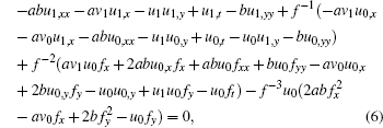
In order to give the concrete expression of u₀, v₀, we substitute Eq. (3) into Eq. (1) and obtain

Vanishing the coefficient of f^{− 3}, we have

Substituting Eq. (8) into Eq. (7) yields the Burgers equation (1b)

Vanishing the coefficient of f^{− 2} in Eq. (6) by using Eq. (8), we have

while the coefficient of f^{− 1} in Eq. (6) equals Eq. (9) by using Eqs. (8) and (10). Finally, vanishing the coefficient of f⁰ in Eq. (6) yields

which is just the Burgers equation (1a) with solutions u₁ and v₁.

Now, using the standard truncated Painlevé expansion

we have the following Bä cklund transformation theorem.

Theorem 1 Transformation (12) is a Bä cklund transformation between solutions {u₁, v₁} and {u, v} if the former is related to f by Eq. (10).

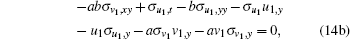
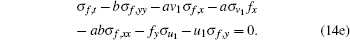
Since u₀ and v₀ are non-local symmetries relating to Bä cklund transformation (3), one can naturally believe that they can be localized to a Lie point symmetry such that we can use Lie’ s first theorem to recover the original Bä cklund transformation. To this end, we introduce new variables to eliminate the space derivatives of f

and investigate the symmetries between different variables. In other words, we have to solve the linearized form of the extended equations (1), (10), (12), and (13)

It can be easily verified that the solution of Eq. (14) has the form

if d₃ is fixed as − 1/(2b).

The result (15) indicates that the residual symmetries (8) are localized in the properly extended system (1), (10), (12), and (13) with the Lie point symmetry vector

In other words, the symmetries related to the truncated Painlevé expansion are just a special Lie point symmetry of the extended system.

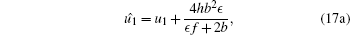
Now we have obtained the localized residual symmetries, an interesting question is what kind of finite transformation would correspond to the Lie point symmetry (16). We have the following theorem.

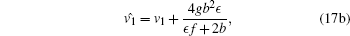
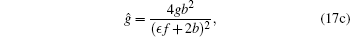
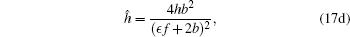
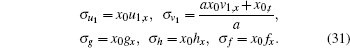
Theorem 2 If {u₁, v₁, g, h, f} is a solution of the extended system (1), (10), (12), and (13), then so is given by

with arbitrary group parameter ϵ .

Proof Using Lie’ s first theorem on vector (16) with the corresponding initial condition

one can easily obtain the solutions of the above equations given in Theorem 2, thus the theorem is proved.

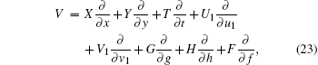
Next let us consider the Lie point symmetry of the extended system in the general form

which means that the extended system (1), (10), (12), and (13) is invariant under the following transformation:

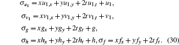
with infinitesimal parameter ϵ . Equivalently, the symmetry in form (23) can be written in a function form

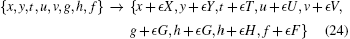
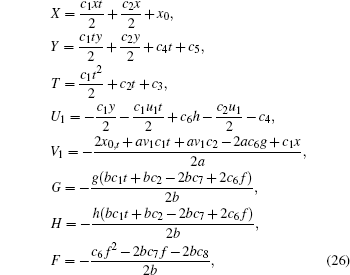
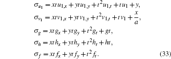
Substituting Eq. (25) into Eq. (14) and eliminating u_{1, t}, v_{1, y}, g_t, h_x, h_t, f_x, f_y, and f_t in terms of the extended system, we obtain more than 250 determining equations for functions X, Y, T, U₁, V₁, G, H, and F. By using a computer algebra, we finally obtain the desired result

with arbitrary constants c₁, c₂, c₃, c₄, c₅, c₆, c₇, c₈ and arbitrary function x₀ of t.

The obtained symmetries can be categorized by different transformation invariances as follows.

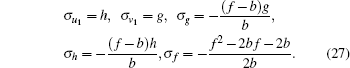
(i) The residual symmetries and and the symmetries relating to the Mö bious transformation can be obtained by setting c₁ = c₂ = c₃ = c₄ = c₅ = x₀ = 0 and c₆ = c₇ = c₈ = − 1

(ii) The symmetries relating to the time transformation can be found by setting c₁ = c₂ = c₄ = c₅ = c₆ = c₇ = c₈ = x₀ = 0 and c₃ = 1

(iii) The symmetries relating to the y-space transformation can be found by setting c₁ = c₂ = c₃ = c₄ = c₆ = c₇ = c₈ = x₀ = 0 and c₅ = 1

(iv) The symmetries relating to the scaling transformation can be found by setting c₁ = c₃ = c₄ = c₅ = c₆ = c₇ = c₈ = x₀ = 0 and c₂ = 2

(v) The symmetries relating to time relevant x-space transformation can be found by setting c₁ = c₂ = c₃ = c₄ = c₅ = c₆ = c₇ = c₈ = 0

(vi) The symmetries relating to the Galileo transformation can be found by setting c₁ = c₂ = c₃ = c₅ = c₆ = c₇ = c₈ = x₀ = 0 and c₄ = 1

(vii) The symmetries relating to the time-Mö bious transformation can be found by setting c₂ = c₃ = c₄ = c₅ = c₆ = c₇ = c₈ = x₀ = 0 and c₁ = 2

Now let us proceed to reduce the extended system by the standard Lie point symmetry group approach. Without loss of generality, we consider the symmetry reductions relating to the space– time invariant and the residual symmetries by setting c₁ = c₂ = c₄ = c₇ = 0 and c₃ = c₅ = c₆ = c₈ = x₀ = 1. Substituting Eq. (26) into Eq. (25) with Eqs. (12) and (13), we obtain

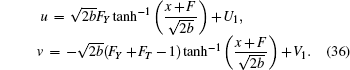
The corresponding group invariant solutions, which can be obtained by solving Eqs. (9)– (11) and (34) with σ _u1 = σ _v1 = σ _f = 0, have the general form

where the group invariant variables are Y = − x + y and T = − x+t, while F, U₁, and V₁ are all group invariant functions of Y and T.

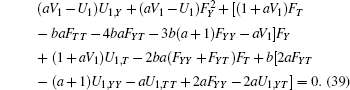
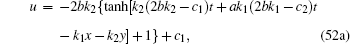
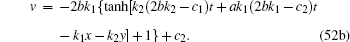
Substituting Eq. (35) into Eq. (12), we obtain the reduction solution for Burgers system (1)

In order to obtain the symmetry reduction equations for the group invariant functions F, U₁, and V₁, we first substitute Eq. (35) into Eq. (9) and find

Next, substituting Eq. (35) into Eq. (10) and vanishing different powers of , we obtain

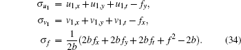
Finally, we obtain three symmetry reduction equations by substituting Eq. (35) into Eq. (11) and vanishing different powers of , two of them are trivial, leaving only the third one

The entrance of the tanh part in Eq. (35) indicates the intrusion of an additional soliton to the background wave. In other words, the group invariant solution (35) is an interaction solution of one soliton and the background wave.

The tanh function is the simplest automorphic function which possesses the property that its derivatives can be explicitly expressed by itself. Enlightened by the form of the reduction solutions of the Burgers equation in Eq. (35), we now use the general tanh function expansion method to study the interaction structure between different solitons.

The general truncated tanh expansion for (2+1)-dimensional Burgers system (1) has the form

where w₁, w₀, p₁, p₀, and ϕ are arbitrary functions of x, y, and t. The λ t in Eq. (40) has been added for later convenience.

Now, by substituting the tanh expansion (40) into the Burgers system (1) and vanishing different powers of tanh(ϕ ) in both expansion equations, we can prove the following Bä cklund transformation theorem.

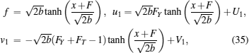
Theorem 3 If f₁ and f₂ are the solution of the Burgers system (1), then so are u and v given by

with

Proof Substituting Eq. (40) into Burgers system (1) with λ = 0 temporarily, we obtain

Vanishing the coefficients of tanh³(ϕ ) in Eq. (43) and tanh²(ϕ ) in Eq. (44), we obtain

The coefficients of tanh²(ϕ ) and tanh(ϕ ) in Eq. (43) are equivalent after using Eq. (45), which reads

After using Eq. (45), equation (44) is degenerated into the Burgers equation (1b)

Vanishing the coefficient of tanh⁰(ϕ ) in Eq. (43), we obtain

with

It can be easily verified that f₁ and f₂ also satisfy

It is obvious that equations (48) and (51) are just the (2+1)-dimensional Burgers system. Substituting w₀ and p₀ by putting Eqs. (49) and (50) into Eq. (46) meanwhile replacing ϕ by λ t + ϕ , we then obtain Eq. (42). Now substituting w₀, p₀, w₁, and p₁ into Eq. (40) by using Eqs. (45), (49), and (50), we finally obtain the Bä cklund transformation (41). The theorem is proved.

If the seed functions are taken as constants, i.e., f₁ = c₁ and f₂ = c₂, then equation (42) becomes a potential Burgers equation with source λ . Even for the seed solutions taken as constants, we can still obtain rich nontrivial solutions from the Bä cklund transformation (41). For instance, the straight line solution ϕ = k₁x+ k₂y = ω t of Eq. (42) leads to the single kink soliton solution

The traveling wave solution of Eq. (42) with f₁ = c₁ and f₂ = c₂ leads to a kink soliton solution

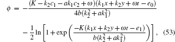
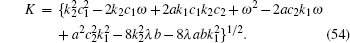
where k₁, k₂, e₀, e₁, and ω are arbitrary constants and K is related to other constants by

Substituting the kink soliton solution (53) into Eq. (41) with f₁ = c₁ and f₂ = c₂, we obtain the two-soliton fusion solution for u and v.

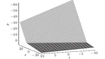
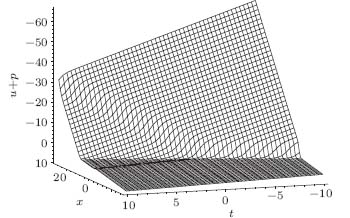
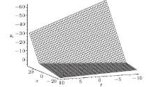
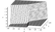
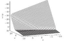
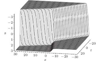
We draw the corresponding figures of Eqs. (53) and (41a) with Eq. (53) and the interaction structure between them by plotting projectively at the y = 1 plane, while the parameters are fixed as

Figure 1 reveals that solution (53) of Eq. (42) is a kink soliton. From Fig. 2, which displays the soliton structure of Eq. (41a), we see that two kink solitons fused to one at some time. Figure 3 displays three solitons interaction structure between u of Eq. (41a) with f₁ = c₁ and ϕ of Eq. (53). It is interesting to find from this picture that three kink solitons fused to one after the interaction. Because the field v of Eq. (41b) resembles u in form, the interaction structure between field v with ϕ of Eq. (53) has the similar form as that in Fig. 3.

Fig. 1.

	Figure Option ViewDownloadNew Window
	Fig. 1. The kink soliton solution (53).

Fig. 2.

	Figure Option ViewDownloadNew Window
	Fig. 2. The two kink solitons fusion structure of u in Eq. (41a) with Eq. (53).

Fig. 3.

	Figure Option ViewDownloadNew Window
	Fig. 3. Evolution of three kink solitons fusion interaction.

In summary, the (2+1)-dimensional Burgers equation is investigated by multiple ways to find the interactions among different nonlinear excitations. The nonlocal residual symmetries which correspond to the generators of the truncated Painlevé expansions are localized in a new prolonged system. The new Bä cklund transformation (Theorem 2) and the symmetry reduction solutions thus are obtained by using the classical Lie point symmetry approach. The reduction solutions reveal that a new soliton is introduced to interact with the background waves. Enlightened by the form of the reduction solutions of the Burgers equation, we further study this system by a new generalized tanh expansion method. With this method, we give a new Bä cklund transformation (Theorem 3) for the Burgers system. From this Bä cklund transformation, we can obtain rich soliton structures even for the constant seed. Especially, two kink solitons fusion structure and the evolution of three kink solitons fusing to one are displayed by plotting projectively. This fact implies that starting from any seed solution, the Bä cklund transformation (Theorem 3) will introduce an additional soliton to the original seed.

In this paper, we have discussed the localization procedure only for one particular nonlocal symmetry, i.e., the residual symmetries. It is obvious that the the same procedure can be executed for other nonlocal symmetries, such as those obtained from the Bä cklund transformation, the bilinear forms, the negative hierarchies, the nonlinearizations, ^{[30, 31]} and the self-consistent sources.^[32] So it would be meaningful to apply this method to various nonlocal symmetries to find rich nonlinear interactive solutions among different excitations.